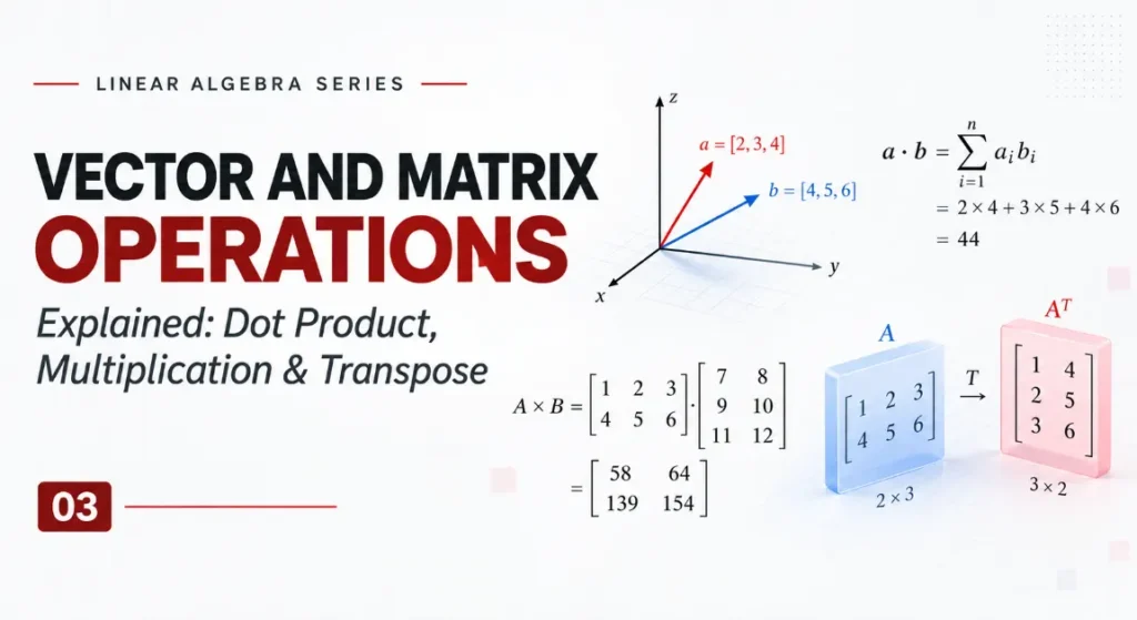
In the previous article, we learned about the basic building blocks of linear algebra: scalars, vectors, and matrices.

We saw that a scalar is a single number, a vector is an ordered collection of numbers, and a matrix is a collection of numbers arranged in rows and columns.

But simply representing information is not enough.

In computer science and artificial intelligence, we constantly need to combine, transform, compare, and manipulate this information.

For example, a machine learning model may need to combine a vector of input features The individual pieces of information provided to a machine learning model as input.
with a set of weights Numerical values that determine how strongly each input feature influences a model’s output. .
An image may be represented as a matrix and transformed into another matrix. Two vectors may need to be compared to see how similar they are.

This is where vector and matrix operations become important.

In this article, we will learn the most important operations step by step:

• Vector addition and subtraction
• Scalar multiplication
• Dot product
• Matrix addition and subtraction
• Matrix multiplication
• Matrix Transpose
• Why these operations matter in AI and computer science

1. Vector Addition

Let’s start with one of the simplest operations.

Suppose we have two vectors: a=[2,3] and b = [4,5]

To add them, we simply add their corresponding elements: a+b=[2+4,  3+5] 

Therefore: a+b=[6,8] 

So vector addition works element by element.

Another example

Suppose: a=[1,2,3]  and: b=[4,5,6] 

Then: a+b=[1+4,  2+5,  3+6] a+b=[5,7,9]

Important rule: Two vectors can be added only when they have the same dimension.

For example: [1,2,3]+[4,5,6] is valid.

But: [1,2,3]+[4,5] is not valid because the vectors have different dimensions.

 

2. Vector Subtraction

Vector subtraction works in exactly the same way.

Suppose: a=[7,5]  and: b=[2,3] 

Then: a−b=[7−2,  5−3] 

Therefore: a−b=[5,2] Again, corresponding elements are operated on individually.

 

3. Scalar Multiplication

We already saw that a scalar is a single number. A scalar can be multiplied by a vector.

Suppose: v=[3,4] and the scalar is: 22

Then: 2v=2[3,4] 

We multiply every element by 2: 2v=[6,8] 

Another example

5[1,2,3]=[5,10,15] 

Scalar multiplication is useful when we want to scale a vector.

For example, if a vector represents a movement of 3 units right and 4 units upward, multiplying it by 2 gives a movement twice as large:

[3,4]→[6,8] This idea becomes important later when we study vectors geometrically.

 

4. The Dot Product

Now we come to one of the most important vector operations in machine learning: the dot product.

Suppose we have: a=[2,3] and: b=[4,5] 

The dot product is calculated by multiplying corresponding elements and then adding the results.

So: a⋅b=(2×4)+(3×5) | 8+15 =23

Therefore: a⋅b=23 

Notice something important. We started with two vectors, but the result is a single scalar.

 

5. Dot Product with Three Elements

Consider: a=[1,2,3]  and: b=[4,5,6] 

Then: a⋅b=(1×4)+(2×5)+(3×6) = 4+10+18 = 32

Therefore: a⋅b=32 

The general idea is:  \[
a \cdot b = \sum_{i=1}^{n} a_i b_i
\]

In simple words: multiply corresponding elements and add the results. 

 

6. Why Is the Dot Product Important in AI?

The dot product appears everywhere in machine learning. Imagine that we have three features describing a house: x=[1200,3,2] 

These could represent:

• Area = 1200
• Bedrooms = 3
• Bathrooms = 2

Now suppose a model has three corresponding weights: w=[0.5,2,1] 

The model can combine the features and weights using a dot product:

\[
w \cdot x = 608
\]

The calculation is:

\[
(0.5 \times 1200) + (2 \times 3) + (1 \times 2)
\]

\[
= 600 + 6 + 2
\]

\[
= 608
\]

This is one of the fundamental ideas behind how machine learning models combine inputs with weights. Later, when we study linear regression and neural networks, this idea will appear repeatedly.

 

7. Vector Operations in Python

We can perform these operations using NumPy.

import numpy as np

a = np.array([2, 3])
b = np.array([4, 5])

print(a + b)
print(a - b)
print(2 * a)
print(np.dot(a, b))

The output is:

[6 8]
[-2 -2]
[4 6]
23

Notice how closely the code follows the mathematics.

 

8. Matrix Addition

Now let’s move from vectors to matrices.

Consider:  A= \begin{bmatrix} 1&2\\ 3&4 \end{bmatrix}

and:  B= \begin{bmatrix} 5&6\\ 7&8 \end{bmatrix}

To add two matrices, we add their corresponding elements.

 A+B= \begin{bmatrix} 1+5&2+6\\ 3+7&4+8 \end{bmatrix}

Therefore:  A+B= \begin{bmatrix} 6&8\\ 10&12 \end{bmatrix}

Just like vectors, matrix addition works element by element.

 

Important rule

Two matrices must have the same dimensions to be added or subtracted.

A \(2 \times 2\) matrix can be added to another \(2 \times 2\) matrix.

But a \(2 \times 2\) matrix cannot be directly added to a \(2 \times 3\) matrix.

 

9. Matrix Subtraction

Matrix subtraction works in the same way.

Suppose:

 A= \begin{bmatrix} 8&7\\ 6&5 \end{bmatrix}

and:

 B= \begin{bmatrix} 2&3\\ 4&1 \end{bmatrix}

Then:

 A-B= \begin{bmatrix} 8-2&7-3\\ 6-4&5-1 \end{bmatrix}

So:

 A-B= \begin{bmatrix} 6&4\\ 2&4 \end{bmatrix} 

 

10. Scalar Multiplication of a Matrix

A scalar can also multiply a matrix.

Suppose:  A= \begin{bmatrix} 1&2\\ 3&4 \end{bmatrix}

Multiplying it by 3 gives:  3A= 3 \begin{bmatrix} 1&2\\ 3&4 \end{bmatrix}

Multiply every element by 3:

 3A= \begin{bmatrix} 3&6\\ 9&12 \end{bmatrix}

Again, the operation is performed element by element.

 

11. Matrix Multiplication

Now we reach one of the most important operations in linear algebra: matrix multiplication.

Unlike matrix addition, matrix multiplication is not done by multiplying corresponding elements.

Consider the two matrices:

\[
A=
\begin{bmatrix}
1&2\\
3&4
\end{bmatrix}
\]

and:

\[
B=
\begin{bmatrix}
5&6\\
7&8
\end{bmatrix}
\]

To calculate \(AB\), we multiply each row of \(A\) by each column of \(B\) using the dot product.

Think of it like this: \[
\text{row of }A
\times
\text{column of }B
=
\text{one element of }AB
\]

So we calculate the four elements of the result one by one.

First element:

Take the first row of \(A\):

\[
[1,2]
\]

and the first column of \(B\):

\[
\begin{bmatrix}
5\\
7
\end{bmatrix}
\]

Multiply the corresponding values and add them:

\[
(1\times5)+(2\times7)
\]

\[
=5+14
\]

\[
=19
\]

So the top-left element is \(19\).

Second element:

Now take the same first row of \(A\), but use the second column of \(B\):

\[
[1,2]
\]

and:

\[
\begin{bmatrix}
6\\
8
\end{bmatrix}
\]

Therefore:

\[
(1\times6)+(2\times8)
\]

\[
=6+16
\]

\[
=22
\]

So the top-right element is \(22\).

Third element:

Now move to the second row of \(A\):

\[
[3,4]
\]

and use the first column of \(B\):

\[
\begin{bmatrix}
5\\
7
\end{bmatrix}
\]

Therefore:

\[
(3\times5)+(4\times7)
\]

\[
=15+28
\]

\[
=43
\]

So the bottom-left element is \(43\).

Fourth element:

Finally, use the second row of \(A\) and the second column of \(B\):

\[
[3,4]
\]

and:

\[
\begin{bmatrix}
6\\
8
\end{bmatrix}
\]

Therefore:

\[
(3\times6)+(4\times8)
\]

\[
=18+32
\]

\[
=50
\]

So the bottom-right element is \(50\).

Putting all four results together:

\[
AB=
\begin{bmatrix}
19&22\\
43&50
\end{bmatrix}
\]

The important thing to remember is:

\[
\boxed{\text{Row of }A\times\text{Column of }B}
\]

Each row-column multiplication gives one element of the resulting matrix.

 

12. The Rule for Matrix Multiplication

There is an important rule you must remember.

If \(A\) has dimensions:

\[
m \times n
\]

and \(B\) has dimensions:

\[
n \times p
\]

then \(AB\) will have dimensions:

\[
m \times p
\]

The inside dimensions must match.

For example:

\[
(2 \times 3)(3 \times 4)
\]

is valid.

The result will be:

\[
2 \times 4
\]

because:

\[
(2 \times 3)(3 \times 4)=(2 \times 4)
\]

But:

\[
(2 \times 3)(2 \times 4)
\]

is not valid because the inside dimensions, 3 and 2, do not match.

 

13. A Simple Way to Remember Matrix Multiplication

Think of it like this:

Rows × Columns → New Matrix

For every position in the resulting matrix:

1. Take one row from the first matrix.
2. Take one column from the second matrix.
3. Multiply corresponding values.
4. Add them together.
5. Put the result in the corresponding position.

This is why the dot product is closely connected to matrix multiplication.

In fact, each element of a matrix product is a dot product between a row and a column. 

 

14. Matrix Multiplication in Python

NumPy makes matrix multiplication straightforward.

import numpy as np

A = np.array([
    [1, 2],
    [3, 4]
])

B = np.array([
    [5, 6],
    [7, 8]
])

C = A @ B

print(C)

Output:

[[19 22]
 [43 50]]

The @ operator is commonly used in Python for matrix multiplication.

 

15. Matrix Multiplication vs Element-Wise Multiplication

This distinction is important.

Suppose:

\[
A=
\begin{bmatrix}
1&2\\
3&4
\end{bmatrix}
\]

and:

\[
B=
\begin{bmatrix}
5&6\\
7&8
\end{bmatrix}
\]

Element-wise multiplication gives:

\[
A\odot B=
\begin{bmatrix}
1\times5&2\times6\\
3\times7&4\times8
\end{bmatrix}
\]

\[
=
\begin{bmatrix}
5&12\\
21&32
\end{bmatrix}
\]

But matrix multiplication gives:

\[
AB=
\begin{bmatrix}
19&22\\
43&50
\end{bmatrix}
\]

 

They are different operations.

In NumPy:

A * B performs element-wise multiplication.

While:

A @ B  performs matrix multiplication.

 

16. Matrix Transpose

Another important operation is the transpose of a matrix.

The transpose changes the rows of a matrix into columns and the columns into rows.

Suppose:

\[
A=
\begin{bmatrix}
1&2&3\\
4&5&6
\end{bmatrix}
\]

This matrix has 2 rows and 3 columns, so it is a \(2\times3\) matrix.

Its transpose is written as:

\[
A^T
\]

and is:

\[
A^T=
\begin{bmatrix}
1&4\\
2&5\\
3&6
\end{bmatrix}
\]

The original matrix was \(2\times3\).

The transpose is \(3\times2\).

So:

\[
(2\times3)^T=(3\times2)
\]

 

 

17. Transpose in Python

With NumPy, we can use .T.

import numpy as np

A = np.array([
    [1, 2, 3],
    [4, 5, 6]
])

print(A.T)

Output:

[[1 4]
 [2 5]
 [3 6]]

18. Why Is Transpose Useful?

Transpose may seem simple, but it is extremely useful in mathematics, statistics, and machine learning.

For example, a vector can be represented as a column:

\[
x=
\begin{bmatrix}
2\\
4\\
6
\end{bmatrix}
\]

Its transpose is:

\[
x^T=
\begin{bmatrix}
2&4&6
\end{bmatrix}
\]

This becomes useful when performing operations where the dimensions need to match.

You will encounter transpose frequently when studying linear regression, covariance matrices, optimization, and machine learning algorithms.

 

19. Vector-Matrix Multiplication.

Let’s take a simple example.

Suppose:

\[
x=
\begin{bmatrix}
2\\
3
\end{bmatrix}
\]

and:

\[
W=
\begin{bmatrix}
1&4\\
2&5
\end{bmatrix}
\]

We can multiply them:

\[
Wx=
\begin{bmatrix}
1&4\\
2&5
\end{bmatrix}
\begin{bmatrix}
2\\
3
\end{bmatrix}
\]

Using row-by-column multiplication:

\[
=
\begin{bmatrix}
(1\times2)+(4\times3)\\
(2\times2)+(5\times3)
\end{bmatrix}
\]

\[
=
\begin{bmatrix}
14\\
19
\end{bmatrix}
\]

This is matrix-vector multiplication. We multiply the matrix WW by the vector xx, using the same row-by-column rule used in matrix multiplication.

This simple operation is already very close to what happens inside machine learning models.

 

20. Matrix Operations Inside Neural Networks

Neural networks perform many operations using vectors and matrices.

Suppose the input to a model is:

\[
x=
\begin{bmatrix}
x_1\\
x_2\\
x_3
\end{bmatrix}
\]

The network can have a weight matrix:

\[
W
\]

and a bias vector:

\[
b
\]

The basic calculation can be written as:

\[
z=Wx+b
\]

This equation is one of the fundamental building blocks of neural networks.

Here:

– \(x\) represents the input.
– \(W\) represents the weights.
– \(b\) represents the bias.
– \(z\) represents the result before an activation function is applied.

Later, when we study neural networks in more detail, we will see how these matrix operations allow a model to process many inputs efficiently.

 

21. Why These Operations Matter in Computer Science

These operations are not just mathematical exercises. They appear in many areas of computer science.

Machine Learning

Vectors represent features and matrices represent collections of data and model parameters.

Neural Networks

Matrix multiplication is used extensively between layers.

Computer Graphics

Matrices can represent transformations such as rotation, scaling, and translation.

Computer Vision

Images can be represented using matrices, while transformations and filters involve matrix operations.

Data Science

Datasets are often represented as matrices where rows represent observations and columns represent features.

Natural Language Processing

Words, sentences, and other language representations can be converted into vectors, and models perform mathematical operations on these representations.

 

Here is summary of what I have written till now.

Operation	What it does
Vector addition	Adds corresponding elements
Vector subtraction	Subtracts corresponding elements
Scalar multiplication	Multiplies every element by a scalar
Dot product	Multiplies corresponding elements and adds them
Matrix addition	Adds corresponding matrix elements
Matrix subtraction	Subtracts corresponding matrix elements
Matrix multiplication	Combines rows and columns
Transpose	Converts rows into columns and columns into rows

The most important ideas to remember are:

Dot product:

\[
a\cdot b=\sum a_i b_i
\]

Matrix multiplication:

\[
(m\times n)(n\times p)=m\times p
\]

Transpose: 

\[
(m\times n)^T=n\times m
\]

 

23. The Bigger Picture

At this point, we have learned the basic objects of linear algebra and how to operate on them.

We started with:

Scalars → Vectors → Matrices

and now we have learned how to:

Add → Subtract → Scale → Multiply → Transpose

These operations form the foundation for much more advanced topics.

When you see an equation such as:

\[
y=Wx+b
\]

it is no longer just a collection of symbols. You can now understand what is happening:

A matrix \(W\) is being multiplied by a vector \(x\), and a bias \(b\) is being added to the result.

This is one of the reasons linear algebra is so important in AI.

In the next article, we will take these ideas into something more practical: systems of linear equations and how Gaussian elimination can be used to solve them.

 

What Comes Next?

Article 4: Systems of Linear Equations and Gaussian Elimination Explained

We will learn:

• What a system of linear equations is
• How equations can be represented using matrices
• Augmented matrices
• Elementary row operations
• Gaussian elimination
• Row echelon form
• How computers solve systems of equations
• Why these ideas matter in computer science and AI

Linear algebra becomes much more interesting when we start using matrices to solve actual problems.