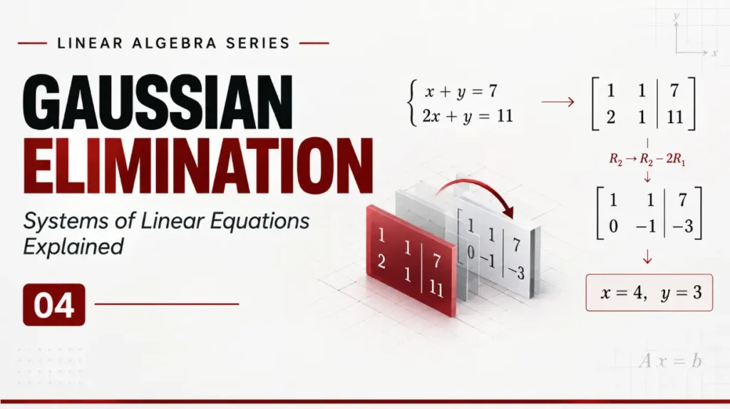
In the previous article, we learned about important vector and matrix operations such as addition, subtraction, scalar multiplication, matrix multiplication, and transpose.

But matrices are not only useful for storing and manipulating numbers. They can also help us represent and solve systems of equations.

For example, consider:

$x+y=7$ and 2x+y=11

We want to find values of $xx$ and $yy$ that satisfy both equations at the same time.

We can solve a small system like this by substitution. But what happens when we have three, ten, or even thousands of variables?

This is where Gaussian elimination, row operations, and row reduction become important.

In this article, we will build the idea step by step:

Linear equations
Systems of linear equations
Substitution
Matrix representation
Augmented matrices
Elementary row operations
Gaussian elimination
Row reduction
Row echelon form
Reduced row echelon form (RREF)
Back substitution
Systems with one, no, or infinitely many solutions
Larger systems
Applications in computer science and AI
Solving systems with Python

1. What Is a Linear Equation?

A linear equation is an equation in which the variables appear only to the first power.

For example:

$x+y=7$

is a linear equation.

So is:

$2x+3y=12$

And:

$x+2y+3z=10$

However, equations such as:

$x^2+y=5$

or:

$xy=10$

are not linear equations because they contain a squared variable or a product of variables.

The word linear is important because linear equations have a structure that allows us to use powerful mathematical tools such as matrices and Gaussian elimination.

2. What Is a System of Linear Equations?

A system of linear equations is a collection of two or more linear equations involving the same variables.

For example:

$x+y=7$

and:

$2x+y=11$

This is a system containing two equations and two unknowns.

We are looking for values of $x$ and $y$ that satisfy **both equations simultaneously**.

We can test a possible solution.

Suppose:

$x=4$

and:

$y=3$

For the first equation:

$4+3=7$

which is true.

For the second equation:

$2(4)+3=11$

which is also true.

Therefore:

$x=4,\qquad y=3$

is the solution of the system.

The important idea is that a solution to a system must satisfy every equation in the system.

3. Why Do We Need Systems of Equations?

Systems of equations appear whenever several unknown quantities are related to one another.

For a simple example, imagine that two unknown quantities must satisfy two different conditions.

One equation describes the first condition, while another describes the second.

Solving only one equation may not be enough to determine all the unknowns. The equations work together to provide the information we need.

For small systems, we can solve them manually.

For example:

$x+y=7$

and:

$2x+y=11$

But as the number of variables increases, manually manipulating equations becomes increasingly difficult.

A system with three variables might look like:

$x+y+z=6$

$2x+y+z=7$

$x+2y+z=8$

And real computational problems can contain hundreds, thousands, or even millions of variables.

We therefore need a systematic method.

4. Solving a System by Substitution

Before introducing matrices, let’s solve a small system using a familiar method: substitution.

Consider:

$x+y=7$

and:

$2x+y=11$

From the first equation:

$y=7-x$

Now substitute this into the second equation:

$2x+(7-x)=11$

Simplify:

$x+7=11$

Therefore:

$x=4$

Now substitute $x=4$ back into:

$y=7-x$

So:

$y=7-4$

Therefore:

$y=3$

The solution is:

$x=4,\qquad y=3$

Substitution works very well for small systems.

But imagine trying to solve a system with 10, 100, or 1,000 variables this way.

The calculations would quickly become difficult to manage. This is where Gaussian elimination becomes useful.

5. Representing a System as a Matrix

Here is where the matrix concepts from the previous articles become useful.

Consider:

$x+y=7$

and:

$2x+y=11$

From the first equation:

$y=7-x$

Now substitute this into the second equation:

$2x+(7-x)=11$

Simplify:

$x+7=11$

Therefore:

$x=4$

Now substitute $x=4$ back into:

$y=7-x$

So:

$y=7-4$

Therefore:

$y=3$

The solution is:

$x=4,\qquad y=3$

Substitution works very well for small systems.

6. The Augmented Matrix

We can make the system even easier to work with.

Instead of separately writing the coefficient matrix, variable vector, and result vector, we can combine the coefficients and results into an augmented matrix.

Our system:

$x+y=7$

and:

$2x+y=11$

becomes:

\[
\left[
\begin{array}{cc|c}
1&1&7\\
2&1&11
\end{array}
\right]
\]

The vertical line separates the coefficients from the results.

The left side:

\[
\begin{bmatrix}
1&1\\
2&1
\end{bmatrix}
\]

contains the coefficients of $x$ and $y$.

The right side contains the constants:

\[
\begin{bmatrix}
7\\
11
\end{bmatrix}
\]

So the augmented matrix gives us a compact representation of the entire system.

More importantly, it gives us a convenient structure on which we can perform row operations.

7. Elementary Row Operations

When solving a system using Gaussian elimination, we manipulate the rows of its augmented matrix.

There are three elementary row operations.

1. Swap two rows

For example:

$R_1\leftrightarrow R_2$

This simply changes their order.

2. Multiply a row by a non-zero number

For example:

$R_1\rightarrow2R_1$

Every element in the first row is multiplied by $2$.

The number cannot be zero because multiplying an entire row by zero would destroy information from that equation.

3. Add or subtract a multiple of one row from another

For example:

$R_2\rightarrow R_2-2R_1$

This means:

Replace $R_2$ with $R_2-2R_1$.

These three operations allow us to transform a system into a simpler form without changing its solution set.

That is the foundation of Gaussian elimination.

8. What Is Gaussian Elimination?

Gaussian elimination is a systematic method for solving systems of linear equations by using elementary row operations to eliminate variables.

The main idea is simple:

Use row operations to create zeros below the leading entries, turning the matrix into a simpler structure.

Let’s use our example again:

\[
\left[
\begin{array}{cc|c}
1&1&7\\
2&1&11
\end{array}
\right]
\]

We want to eliminate the $2$ below the first $1$.

We perform:

$R_2\rightarrow R_2-2R_1$

The new second row is:

\[
[2,1,11]-2[1,1,7]
\]

First calculate:

\[
2[1,1,7]=[2,2,14]
\]

Therefore:

\[
[2,1,11]-[2,2,14]=[0,-1,-3]
\]

So our matrix becomes:

\[
\left[
\begin{array}{cc|c}
1&1&7\\
0&-1&-3
\end{array}
\right]
\]

The second row represents:

$-y=-3$

Therefore:

$y=3$

Now substitute $y=3$ into the first equation:

$x+y=7$

$x+3=7$

Therefore:

$x=4$

So:

$x=4,\qquad y=3$

This is Gaussian elimination in action.

9. Why Is It Called “Elimination”?

The name comes directly from what we are doing.

We are eliminating variables from the equations.

Initially:

$x+y=7$

$2x+y=11$

Both equations contain $x$.

After applying:

$R_2\rightarrow R_2-2R_1$

we obtain:

$x+y=7$

$-y=-3$

The $x$ has been eliminated from the second equation.

Once a variable has been eliminated, the remaining variables become easier to determine.

For larger systems, we continue this process until the matrix reaches a structured form.

10. Row Reduction

Row reduction refers to the process of using elementary row operations to transform a matrix into a simpler form.

Gaussian elimination is one important application of row reduction.

For example, suppose we have:

\[
\left[
\begin{array}{ccc|c}
1&2&3&10\\
2&5&8&23\\
1&1&2&7
\end{array}
\right]
\]

We can use elementary row operations to eliminate entries below the leading entries.

The goal is not to randomly change numbers.

Instead, each operation moves the matrix toward a more useful structure.

Depending on how far we continue the reduction, we may obtain row echelon form or reduced row echelon form.

11. Row Echelon Form (REF)

A matrix is in row echelon form, or REF, when it has a staircase-like structure.

The important rules are:

All rows containing only zeros are at the bottom.
The first non-zero entry in each non-zero row is to the right of the first non-zero entry in the row above it.
All entries below each leading entry are zero.

For example:

\[
\left[
\begin{array}{ccc|c}
1&2&3&10\\
0&1&4&8\\
0&0&1&5
\end{array}
\right]
\]

is in row echelon form.

Notice the staircase:

The first leading entry is in column 1.
The next leading entry is farther to the right.
The third leading entry is farther to the right again.
Everything below each leading entry is zero.

This structure allows us to solve the system from the bottom upward.

That process is called back substitution.

12. Reduced Row Echelon Form (RREF)

We can take row reduction one step further.

A matrix is in reduced row echelon form, or RREF, when it satisfies stricter conditions.

The rules are:

Rule 1: All zero rows are at the bottom

For example:

\[
\begin{bmatrix}
1&2&3\\
0&1&4\\
0&0&0
\end{bmatrix}
\]

The zero row is at the bottom.

Rule 2: Every leading entry is 1

For example:

\[
\begin{bmatrix}
1&2&3\\
0&1&4
\end{bmatrix}
\]

The leading entries are both $1$.

A leading $11$ is often called a pivot.

Rule 3: Each pivot is the only non-zero entry in its column

For example:

\[
\begin{bmatrix}
1&0&5\\
0&1&4
\end{bmatrix}
\]

The first pivot is the $1$ in column 1, and every other entry in that column is zero.

The second pivot is the $1$ in column 2, and every other entry in that column is zero.

Rule 4: Each pivot is to the right of the pivot above it

For example:

\[
\begin{bmatrix}
1&2&0&5\\
0&1&3&4\\
0&0&1&2
\end{bmatrix}
\]

The pivots move progressively to the right as we move downward.

This gives the matrix its staircase structure.

REF vs RREF

The distinction is important.

In REF, we make the entries below each pivot zero.

In RREF, we go further and make the entries above and below each pivot zero, while also making every pivot equal to $11$ .

For example, this is REF:

\[
\begin{bmatrix}
1&2&3\\
0&1&4\\
0&0&1
\end{bmatrix}
\]

while this is RREF:

\[
\begin{bmatrix}
1&0&0\\
0&1&0\\
0&0&1
\end{bmatrix}
\]

RREF gives us an especially clean representation of the solution structure.

13. Gaussian Elimination Step by Step

Let’s now go through a complete example.

Consider:

$x+y=7$

$2x+y=11$

Write the augmented matrix:

\[
\left[
\begin{array}{cc|c}
1&1&7\\
2&1&11
\end{array}
\right]
\]

We want to eliminate the $2$ below the first pivot.

Perform:

$R_2\rightarrow R_2-2R_1$

This gives:

\[
\left[
\begin{array}{cc|c}
1&1&7\\
0&-1&-3
\end{array}
\right]
\]

This is already in row echelon form.

We can now use back substitution.

The second row gives:

$-y=-3$

Therefore:

$y=3$

Substitute into the first row:

$x+y=7$

$x+3=7$

Therefore:

$x=4$

So the solution is:

$x=4,\qquad y=3$

14. Back Substitution

Back substitution is the process of solving for variables starting from the last equation and then substituting those values into the equations above.

Consider the system represented by:

\[
\left[
\begin{array}{ccc|c}
1&2&3&10\\
0&1&4&8\\
0&0&1&5
\end{array}
\right]
\]

The last row gives:

$z=5$

Now move to the second row:

$y+4z=8$

Substitute $z=5$:

$y+20=8$

Therefore:

$y=-12$

Now use the first row:

$x+2y+3z=10$

Substitute:

$x+2(-12)+3(5)=10$

Simplify:

$x-24+15=10$

Therefore:

$x=19$

So the solution is:

$x=19,\qquad y=-12,\qquad z=5$

This illustrates why row echelon form is useful: once the system has been reduced to a staircase structure, we can work upward to find the variables.

15. One Solution, No Solution, or Infinitely Many Solutions

A system of linear equations does not always have exactly one solution.

There are three important possibilities.

One solution

A system has one solution when the equations determine one unique combination of variables.

For example:

$x+y=7$

and:

$x-y=1$

These equations intersect at one point, giving one solution.

No solution

A system can also be contradictory.

Consider:

$x+y=5$

and:

$x+y=8$

The same expression cannot equal both $5$ and $8$.

Therefore, the system has no solution.

During row reduction, this type of contradiction can appear as:

\[
\left[
\begin{array}{cc|c}
0&0&3
\end{array}
\right]
\]

which represents:

$0=3$

This is impossible.

Infinitely many solutions

Sometimes the equations do not provide enough independent information to determine one unique solution.

For example:

$x+y=5$

and:

$2x+2y=10$

The second equation is simply twice the first.

Therefore, both equations describe the same relationship.

There are infinitely many pairs $(x,y)$ that satisfy them.

In row-reduced form, this type of situation can appear when at least one variable remains free.

16. Gaussian Elimination in Larger Systems

The real advantage of Gaussian elimination becomes clearer when we have more variables.

Consider:

$x+y+z=6$

$2x+y+z=7$

$x+2y+z=8$

Instead of repeatedly substituting equations into one another, we can write:

\[
\left[
\begin{array}{ccc|c}
1&1&1&6\\
2&1&1&7\\
1&2&1&8
\end{array}
\right]
\]

We can then systematically perform row operations to eliminate entries below the pivots.

The same basic process works for systems containing many more variables.

This scalability is one of the reasons Gaussian elimination is such an important idea in linear algebra.

17. Systems of Equations in Computer Science

Systems of linear equations are not limited to classroom mathematics.

They appear in many areas of computer science, engineering, and data analysis.

Computer Graphics

Linear equations can be used when calculating intersections, transformations, and geometric relationships.

Computer Vision

Systems of equations can appear when estimating information about objects, cameras, and three-dimensional scenes from images.

Machine Learning

Many mathematical problems in machine learning involve solving or approximating systems of equations.

Data Science

Linear regression and other statistical techniques rely heavily on linear algebra and related systems.

Engineering and Simulation

Physical systems can involve many interacting variables. These relationships can often be represented using systems of equations and solved computationally.

The important idea is that computers can handle systems containing far more variables than would be practical to solve manually.

18. Gaussian Elimination in Python

We can also solve systems of equations computationally using Python and NumPy.

For example:

import numpy as np

A = np.array([
    [1, 1],
    [2, 1]
])

b = np.array([7, 11])

x = np.linalg.solve(A, b)

print(x)

Output:

[4. 3.]

The result tells us:

$x=4,\qquad y=3$

The important thing to understand is that a library such as NumPy allows us to obtain the solution without manually performing every row operation.

However, learning the underlying mathematics helps us understand what the computer is actually solving.

19. Why This Matters for AI

At this point, we can see a progression through our linear algebra series.

We started with:

Scalars → Vectors → Matrices

Then we learned how to perform operations such as:

Addition → Multiplication → Transpose

Now we are using matrices to represent and solve systems of equations.

This progression is important because modern AI and machine learning rely heavily on these mathematical structures.

A machine learning model may involve a large number of parameters and relationships between variables. Working with these relationships efficiently requires mathematical structures and algorithms that can operate on large collections of numbers.

Gaussian elimination is one of the fundamental methods that helps us understand how systems of equations can be handled systematically.

The deeper lesson is not simply how to perform a particular calculation.

It is learning how to take a complicated mathematical problem, represent it in a structured way, and then simplify that structure step by step.

20. Quick Summary

Let’s summarize what we learned.

A linear equation contains variables only to the first power.
A system of linear equations contains multiple linear equations involving the same variables.
The solution must satisfy every equation in the system.
A system can have one solution, no solution, or infinitely many solutions.
A system can be represented compactly as $Ax=bA\mathbf{x}=\mathbf{b}$ .
An augmented matrix combines the coefficients and results of a system.
Elementary row operations allow us to transform a system while preserving its solution set.
Gaussian elimination systematically eliminates variables using row operations.
Row reduction transforms a matrix into a simpler form.
Row echelon form (REF) creates a staircase structure with zeros below pivots.
Reduced row echelon form (RREF) goes further: pivots are $11$ , each pivot is the only non-zero entry in its column, pivots move to the right as we move downward, and zero rows appear at the bottom.
Back substitution can be used after Gaussian elimination to determine unknown variables.
Larger systems can be handled using the same fundamental process.
Python libraries such as NumPy can solve systems computationally.

The central idea is simple:

Turn equations into a structured form, simplify them systematically, and use that structure to find the unknowns.

The Bigger Picture

Linear algebra becomes much more interesting when we stop looking at equations individually and start seeing the structure connecting them.

A system such as:

$x+y=7$

$2x+y=11$

can be written compactly as:

$A\mathbf{x}=\mathbf{b}$

That small expression connects equations, vectors, and matrices into one mathematical framework.

We can then use row operations to transform that system into increasingly simpler forms, eventually revealing its solution.

This is an important transition in our linear algebra journey.

We have learned how matrices can represent systems and how row operations can solve them.

In the next article, we will look at another important property of matrices: the determinant.

We will explore what a determinant means, how the $2\times2$ and $3\times3$ determinant rules work, how minors and cofactors are formed, why the $+,-,+$ sign pattern appears, and how determinants are connected to the behavior of a matrix.

Systems of Linear Equations and Gaussian Elimination

1. What Is a Linear Equation?

2. What Is a System of Linear Equations?

3. Why Do We Need Systems of Equations?

4. Solving a System by Substitution

5. Representing a System as a Matrix

6. The Augmented Matrix

7. Elementary Row Operations

1. Swap two rows

2. Multiply a row by a non-zero number

3. Add or subtract a multiple of one row from another

8. What Is Gaussian Elimination?

9. Why Is It Called “Elimination”?

10. Row Reduction

11. Row Echelon Form (REF)