Types of Data Structures: A Complete Overview

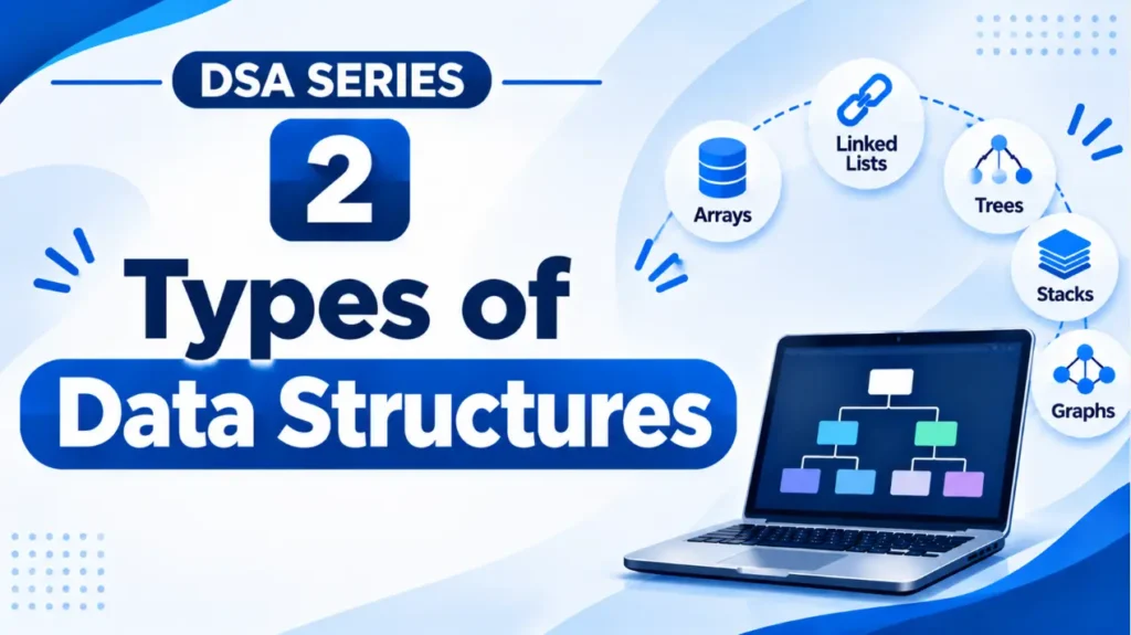
In our previous article, we learned that data structures are different ways of organizing and storing information so that we can work with it efficiently.

We also introduced some common examples, including arrays, linked lists, stacks, queues, trees, and graphs.

But why do we have so many different types? And how do we decide which one to use?

Let’s take a practical example.

Imagine you are developing a university management system. The system needs to handle several things:

• Store the marks of thousands of students.
• Maintain a list of students enrolled in different courses.
• Manage students waiting for registration.
• Represent the hierarchy of university departments.
• Store connections between students and the courses they have selected.
• Find a student’s record using their registration number.

Would you use the same method to organize all this information? Probably not.

Storing marks is different from managing a waiting line, and representing a university’s organizational structure is different from finding a student’s record.

Each task has different requirements. This is why we have different data structures.

Let’s understand how they are classified.

1. Classification of Data Structures

Data structures can be classified in several ways, depending on how they organize information and manage memory.

The most common introductory classifications are:

1. Primitive and Non-Primitive Data Structures
2. Linear and Non-Linear Data Structures
3. Static and Dynamic Data Structures

These classifications describe different characteristics. For example, a structure can be linear and dynamic at the same time.

Let’s understand each classification.

2. Primitive and Non-Primitive Data Structures

The first classification is based on the kind of data being represented and how complex its organization is.

A. Primitive Data Types

Primitive data types are the basic types provided by a programming language. They represent individual values and are used as building blocks for more complex structures.

Common examples include:

1. Integer (int)

Used to store whole numbers.

int age = 20;
int marks = 85;

2. Float (float)

Used to store numbers with decimal values.

float price = 99.50;
float temperature = 36.5;

3. Character (char)

Used to store a single character.

char grade = 'A';

4. Boolean (bool)

Used to represent two logical values: true or false.

bool isPassed = true;

5. Pointer

A pointer is a variable that stores the memory address of another variable or object. Pointers are particularly important in languages such as C and C++.

int number = 10;
int *ptr = &number;

Here, ptr stores the address of number.

The exact set of primitive types varies between programming languages. For example, Python handles integers and strings differently from C.

B. Non-Primitive Data Structures

Non-primitive data structures organize multiple values or represent more complex relationships between data. They are generally built using basic data types and other programming language features.

Some common examples are:

• Arrays
• Strings
• Linked Lists
• Stacks
• Queues
• Trees
• Graphs
• Hash Tables
• Heaps

For example, consider the following array:

int marks[5] = {78, 91, 65, 84, 72};

Instead of creating five separate variables, we organize all five marks under one array.

For example, a linked list stores data in separate small units called nodes. Each node contains some information and a link that connects it to the next node, forming a chain of data.

A stack stores elements one on top of another, like a pile of plates. You can add a new element to the top, and when removing an element, you always remove the top one first.

A tree organizes information into different levels, much like a family tree. For example, a university may have different departments, and each department may have several courses. This arrangement, where information is organized from a main point into smaller related parts, is called a hierarchical structure.

In simple terms: Primitive types represent basic individual values, while non-primitive structures help organize collections of values and more complex relationships.

One thing to remember:
this is a commonly used introductory classification. In modern programming languages, the exact distinction between primitive types, objects, and data structures can vary. We will discuss this more carefully in Article 4, Data Types, Objects, and Data Structures: Representation and Implementation.

3. Linear Data Structures

A linear data structure is one in which elements are organized in a sequential arrangement.

In this arrangement, elements follow a logical order. Except for the first and last elements, each element has a predecessor and a successor in the sequence.

Think about people standing in a queue at a ticket counter. The first person is followed by the second, the second by the third, and so on.

A simplified representation looks like this: [10] → [20] → [30] → [40] → [50]

The elements are arranged one after another. Let’s look at the major linear data structures.

A. Arrays

An array stores multiple elements of the same data type under one variable name. In a typical array implementation, elements occupy consecutive memory locations and can be accessed using an index.

For example: int numbers[5] = {10, 20, 30, 40, 50};

Its logical representation is:

Index:    0    1    2    3    4

        ┌────┬────┬────┬────┬────┐
Value:  │ 10 │ 20 │ 30 │ 40 │ 50 │
        └────┴────┴────┴────┴────┘

Each element has an index, starting from 0 in C, C++, Java, and Python.

For example, numbers[2] gives us 30.

Arrays are useful when we need to store related values and access them by their positions.

Where are arrays used?

• Storing student marks.
• Recording daily temperatures.
• Managing product prices.
• Representing matrices.
• Storing collections of numerical data.

We will study one-dimensional arrays, two-dimensional arrays, matrix operations, and their limitations in Articles 5, 6, and 7.

B. Strings

A string is a sequence of characters used to represent text. For example: "VARIABLE"

We can visualize it as:

┌───┬───┬───┬───┬───┬───┬───┬───┐
│ V │ A │ R │ I │ A │ B │ L │ E │
└───┴───┴───┴───┴───┴───┴───┴───┘

Strings are used whenever a program needs to work with text.

Where are strings used?

• Storing names and addresses.
• Writing messages.
• Processing passwords.
• Searching words in documents.
• Managing website content.

In C, a string is traditionally represented as an array of characters ending with a special null character ('\0'). Other programming languages use different internal representations.

We will explore string representation and operations in Article 8.

C. Linked Lists

A linked list is a linear data structure made up of individual elements called nodes.

Each node stores data and one or more links that connect it to other nodes.

Unlike a traditional array, linked-list nodes do not need to be stored in consecutive memory locations.

For example:

┌───────┬───────┐    ┌───────┬───────┐
│  10   │   •───┼───→│  20   │   •───┼───→ ...
└───────┴───────┘    └───────┴───────┘

Each node points to the next node, forming a chain.

Linked lists are useful when we need to insert or remove elements without shifting all subsequent elements, although accessing a particular position requires following the links.

Where are linked lists used?

• Implementing certain types of playlists.
• Managing sequences of tasks.
• Implementing stacks and queues.
• Maintaining collections where insertions and deletions are frequent.

We will study linked lists, their operations, and their different types in Articles 9 and 10.

D. Stacks

A stack is a linear data structure that follows the principle of LIFO (Last In, First Out). This means the last element added to the stack is the first one removed.

Think about a stack of plates.

When you place plates on top of each other, you usually remove the top plate first.

A stack works in the same way.

        ┌────────┐
        │   30   │ ← TOP
        ├────────┤
        │   20   │
        ├────────┤
        │   10   │
        └────────┘

Here, 30 was added last, so it will be removed first.

Two important operations are:

• Push: Adds an element to the top.
• Pop: Removes the top element.

Stacks are commonly used in:

• Undo and redo operations.
• Browser navigation.
• Function calls and recursion.
• Expression evaluation.
• Checking balanced parentheses.

We will explore stacks and their applications in Articles 15 and 16.

E. Queues

A queue is a linear data structure that follows the principle of FIFO (First In, First Out).

This means the first element added is the first one removed.

Think about people waiting in line at a ticket counter. The person who arrives first is generally served first.

A queue works similarly.

FRONT                         REAR
  ↓                             ↓
┌────┬────┬────┬────┐
│ 10 │ 20 │ 30 │ 40 │
└────┴────┴────┴────┘
  ↑                             ↑
Remove                          Add

Two important operations are:

• Enqueue: Adds an element at the rear.
• Dequeue: Removes an element from the front.

Queues are commonly used in:

• Printer job scheduling.
• Customer service systems.
• Server request processing.
• Task scheduling.
• Managing waiting lists.

We will study queues, circular queues, deques, and priority queues in Articles 17 and 18.

4. Non-Linear Data Structures

Unlike linear data structures, non-linear data structures organize data through hierarchical or network-like relationships. An element may be connected to multiple other elements rather than simply following one sequence.

Consider the organizational structure of a university:

                University
                    |
          ┌─────────┴─────────┐
          |                   |
      Academics          Administration
          |
      ┌───┴────┐
      |        |
   Science  Commerce

Here, information is organized into different levels rather than one simple sequence.

The major non-linear data structures include trees and graphs.

A. Trees

A tree is a non-linear data structure that organizes information hierarchically through nodes connected by edges. It begins with a special node called the root, from which other nodes branch out.

Consider this example:

             A
           /   \
          B     C
         / \   / \
        D   E F   G

Here:

• A is the root node.
• B and C are children of A.
• D and E are children of B.
• F and G are children of C.
• D, E, F, and G are leaf nodes because they have no children.

This is a simple binary tree.

Trees are particularly useful when information has a hierarchical relationship.

Where are trees used?

• Folder and file systems.
• Organizational charts.
• Database indexing.
• HTML document structure (DOM).
• Searching and organizing information.

Some important types of trees include binary trees, binary search trees, AVL trees, B-trees, and B+ trees.

We will explore these structures in detail in Articles 21–24.

B. Graphs

A graph is a non-linear data structure consisting of vertices (also called nodes) and edges that connect them.

Graphs are useful for representing relationships and connections between different objects.

Imagine a simplified social network:

       A ───── B
       |     / |
       |   /   |
       C ───── D

Here:

• A, B, C, and D represent people.
• The lines represent connections between them.

Graphs are not limited to social networks. They can represent many real-world systems.

Where are graphs used?

• Road networks connecting cities.
• Social media connections.
• Computer networks.
• Flight routes between airports.
• Relationships between web pages.

Graphs can be directed or undirected, weighted or unweighted. For example, in a road network, an edge might carry a weight representing the distance between two cities.

We will study graph representations, BFS, DFS, shortest paths, and minimum spanning trees in Articles 25 and 26.

5. Some Other Important Data Structures

Apart from the basic linear and non-linear structures, there are other specialized data structures that are designed for particular operations.

Two important examples are heaps and hash tables.

A. Heaps

A heap is a specialized tree-based data structure that follows a particular ordering rule called the heap property.

There are two common types.

1. Min Heap

In a min heap, the value of every parent node is less than or equal to the values of its children.

           10
          /  \
         20   30
        / \
       40  50

The smallest element is always at the root.

2. Max Heap

In a max heap, the value of every parent node is greater than or equal to the values of its children.

           50
          /  \
         40   30
        / \
       10  20

The largest element is always at the root.

Where are heaps used?

• Priority-based task scheduling.
• Implementing priority queues.
• Heap sort.
• Shortest-path algorithms.

An interesting point is that although heaps are tree-based structures, they are commonly implemented using arrays.

We will explore their representation and implementation in Article 19.

B. Hash Tables

A hash table is a data structure that stores information in key-value pairs and uses a hash function to determine where a value should be stored.

Imagine a university database containing thousands of student records. You want to find a student’s information using their registration number.

A hash table can use that registration number as a key to locate the associated record.

For example:

Key                 Value
--------------------------------
101                 Farhan
102                 Aamir
103                 Danish
104                 Ahmad

A hash function processes a key and calculates an index where its corresponding value can be stored.

The basic process looks like this:

Registration Number
        |
        v
   Hash Function
        |
        v
   Calculated Index
        |
        v
   Stored Record

Hash tables are useful for:

• Dictionaries and maps.
• Database lookups.
• Caching.
• Finding records using unique identifiers.
• Counting the frequency of words.

Sometimes, two different keys produce the same index. This situation is called a collision.

We will study hash functions, collision resolution, chaining, and open addressing in Articles 28 and 29.

6. Static and Dynamic Data Structures

So far, we have classified data structures based on how they organize information.

Now let’s look at another important distinction: how their size or capacity changes during program execution.

This gives us two commonly taught categories: static and dynamic data structures.

A. Static Data Structures

A static data structure has a fixed size or capacity determined when it is created.

For example:

int numbers[5] = {10, 20, 30, 40, 50};

Here, the array has a capacity of five integers.

We cannot simply increase its declared capacity by adding another element to the same array.

Advantages:

• Simple to implement.
• Predictable memory requirements.
• Direct access to elements in arrays.

Limitations:

• Fixed capacity.
• May waste allocated space if it is not fully used.
• Cannot automatically grow beyond its declared capacity.

B. Dynamic Data Structures

A dynamic data structure can change its size during program execution by allocating or releasing memory as required.

For example, a linked list can grow when new nodes are inserted and shrink when nodes are deleted.

Initially:

[10] → [20] → NULL

After inserting 30:

[10] → [20] → [30] → NULL

After deleting 20:

[10] → [30] → NULL

Advantages:

• Flexible size.
• Memory can be allocated when needed.
• Useful when the number of elements is not known in advance.

Limitations:

• Requires additional memory management.
• Some structures need extra memory for pointers or links.
• Implementation can be more complicated.

An important distinction: Static and dynamic describe how memory or capacity is managed. They are not completely separate families of data structures.

For example, a traditional fixed-size array is static, while a linked list is generally dynamic. However, dynamic arrays can also grow when necessary, and a stack can be implemented using either a fixed-size array or a dynamically growing structure.

7. How Do We Choose the Right Data Structure?

Now that we have explored the different types, let’s return to our university management system.

Suppose you are developing it and need to decide how to organize different types of information.

Which structure would you choose?

Requirement	Suitable Data Structure	Reason
Store students’ marks	Array	Organizes values by index
Manage browser undo history	Stack	The most recent action is undone first
Manage students waiting for registration	Queue	First arrival is served first
Represent university departments	Tree	Represents hierarchical relationships
Represent connections between cities	Graph	Represents networks and connections
Find student records using registration numbers	Hash Table	Supports efficient key-based lookup
Retrieve the highest-priority task	Heap	Keeps the highest-priority element accessible

Notice that there is no single data structure suitable for every task.

The choice depends on what you need to do with the data.

For example, if you frequently access elements by their position, an array may be a good choice.

If you need to manage tasks according to priority, a heap may be more suitable.

If you need to represent relationships between multiple objects, a graph may be the right choice.

The important thing is to understand the problem before choosing the data structure.

Conclusion

We have now explored the major types of data structures and how they are classified.

Some organize information sequentially, such as arrays, linked lists, stacks, and queues. Others organize data through hierarchical or network-like relationships, such as trees and graphs.

We also looked at specialized structures such as heaps and hash tables, along with the distinction between static and dynamic memory management.

Each structure has its own advantages, limitations, and suitable applications.

You don’t need to use the most complicated structure to solve a problem. You need to understand what the problem requires and choose a structure that makes the required operations efficient.

In the next article, we will move from understanding different data structures to measuring efficiency.

We will study Space and Time Complexity in DSA, where we will learn how to analyze the time and memory an algorithm requires as the amount of input increases.

DSA Series: Table of Contents

1. What Is DSA? — Completed
2. Types of Data Structures: A Complete Overview — Current Article
3. Space and Time Complexity in DSA
4. Data Types, Objects, and Data Structures: Representation and Implementation
5. Arrays: Understanding the Basics
6. Two-Dimensional Arrays, Matrix Operations, and Sparse Matrices
7. Limitations and Applications of Linear Arrays
8. Strings: Understanding String Data
9. Linked Lists: How They Work (Types and Operations)
10. Singly, Doubly, and Circular Linked Lists: A Deep Dive
11. Linear Search vs. Binary Search
12. Bubble Sort, Selection Sort, and Insertion Sort
13. Merge Sort and Quick Sort: A Comparative Guide
14. Searching and Sorting Algorithms Compared
15. Stack Data Structure: Understanding LIFO
16. Applications of Stacks: Parenthesis Checker, Infix to Postfix, and Evaluation
17. Queue Data Structure: Understanding FIFO
18. Circular Queues, Deques, and Priority Queues
19. Heaps: Representation and Implementation of Priority Queues
20. Recursion: Understanding the Basics
21. Trees: Definitions, Terminologies, and Properties
22. Binary Trees: Representation, Traversals, and Applications
23. Threaded Binary Trees, AVL Trees, and M-Way Search Trees
24. B-Trees and B+ Trees: A Complete Guide
25. Graphs: Terminology, Representations, and Traversal Techniques (BFS & DFS)
26. Minimum Spanning Trees and Shortest Path Algorithms
27. Eulerian Tour and Hamiltonian Tour
28. Hashing: Direct Address Tables, Hash Functions, and Collision Resolution
29. Resolving Collisions: Chaining and Open Addressing (Rehashing)
30. Conclusion