
Articles / Linear Algebra · Part 17
Kernel and Image of Linear Transformations
Understand the kernel and image of linear transformations, how to calculate them using matrices, and how they relate to rank, nullity, injectivity, and surjectivity.

1. Introduction
A linear transformation maps vectors from one vector space to another while preserving vector addition and scalar multiplication.
However, not every vector behaves the same way under a transformation. Some vectors may become the zero vector, while others may be mapped to different vectors in the output space.
To understand this behavior, we study two important concepts:
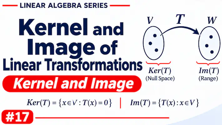
- Kernel (Null Space): The set of all vectors that are mapped to the zero vector.
- Image (Range): The set of all possible outputs produced by the transformation.
These concepts help us understand the structure, behavior, and properties of linear transformations.
2. Kernel of a Linear Transformation
The kernel of a linear transformation is the set of all vectors in its domain that are mapped to the zero vector in its codomain.
If \(T:V\rightarrow W\) is a linear transformation, its kernel is defined as:
\[
\ker(T)={v\in V:T(v)=0_W}
\]
Here, \(0_W\) represents the zero vector in the codomain.
Example
Consider the transformation:
\[
T(x,y)=(x+y,2x+2y)
\]
To find its kernel, we need to determine all vectors that produce the zero vector.
Therefore:
\[
T(x,y)=(0,0)
\]
This gives us the equations:
\[
\begin{aligned}
x+y&=0\\
2x+2y&=0
\end{aligned}
\]
The second equation is simply twice the first, so we only need:
\[
x+y=0
\]
Rearranging:
\[
x=-y
\]
Let (y=t). Then (x=-t).
Therefore, every vector in the kernel has the form:
\[
t\begin{bmatrix}
-1\\1
\end{bmatrix}
\]
Hence:
\[
\boxed{
\ker(T)=
\operatorname{span}
\left\{
\begin{bmatrix}
-1\\1
\end{bmatrix}
\right\}
}
\]
The kernel contains all scalar multiples of the vector ((-1,1)), including the zero vector.
3. Understanding the Kernel Geometrically
The kernel tells us which directions in the input space are completely lost during the transformation.
In our example, consider the vector:
\[
\begin{bmatrix}
1\\-1
\end{bmatrix}
\]
Applying the transformation:
\[
T(1,-1)=(1-1,2-2)=(0,0)
\]
This vector disappears during the transformation.
In fact, every vector along the line \(y=-x\) is mapped to the origin.
This means the transformation loses information about movement along that direction.
4. Image of a Linear Transformation
The image of a linear transformation is the set of all possible outputs that the transformation can produce.
It is also called the range of the transformation.
For \(T:V\rightarrow W\), the image is defined as:
\[
\operatorname{Im}(T)={T(v):v\in V}
\]
In simple words, the image contains every vector that can be obtained by applying the transformation to some input vector.
Example
Again, consider:
\[
T(x,y)=(x+y,2x+2y)
\]
Let:
\[
u=x+y
\]
Then the output becomes:
\[
T(x,y)=(u,2u)
\]
Therefore, every possible output has the form:
\[
u\begin{bmatrix}
1\\2
\end{bmatrix}
\]
Hence:
\[
\boxed{
\operatorname{Im}(T)=
\operatorname{span}
\left\{
\begin{bmatrix}
1\\2
\end{bmatrix}
\right\}
}
\]
The image is the line passing through the origin in the direction of ((1,2)).
Although the transformation takes inputs from \(\mathbb R^2\), its outputs lie only along one line in \(\mathbb R^2\).
5. Finding the Kernel and Image Using a Matrix
Linear transformations can be represented using matrices.
Our transformation:
\[
T(x,y)=(x+y,2x+2y)
\]
can be written as:
\[
T(\mathbf{x})=A\mathbf{x}
\]
where:
\[
A=
\begin{bmatrix}
1&1\\
2&2
\end{bmatrix}
\]
and:
\[
\mathbf{x}=
\begin{bmatrix}
x\\y
\end{bmatrix}
\]
Finding the Kernel
The kernel consists of vectors satisfying:
\[
A\mathbf{x}=\mathbf{0}
\]
Therefore:
\[
\begin{bmatrix}
0\\0
\end{bmatrix}
\]
This gives:
\[
x+y=0
\]
Solving this equation gives:
\[
\ker(T)=
\operatorname{span}
\left\{
\begin{bmatrix}
-1\\1
\end{bmatrix}
\right\}
\]
Finding the Image
The image of a matrix transformation is the column space of its matrix.
The columns of (A) are:
\[
\begin{bmatrix}
1\\2
\end{bmatrix},
\qquad
\begin{bmatrix}
1\\2
\end{bmatrix}
\]
Since both columns are identical, only one independent column exists.
Therefore:
\[
\operatorname{Im}(T)=
\operatorname{span}
\left\{
\begin{bmatrix}
1\\2
\end{bmatrix}
\right\}
\]
This is the column space of (A).
6. Kernel, Image, Rank, and Nullity
The kernel and image are closely connected to two important concepts:
Rank
The rank of a linear transformation is the dimension of its image.
\[
\operatorname{rank}(T)=\dim(\operatorname{Im}(T))
\]
It tells us how many independent directions the transformation can produce in the output space.
Nullity
The nullity of a linear transformation is the dimension of its kernel.
\[
\operatorname{nullity}(T)=\dim(\ker(T))
\]
It tells us how many independent directions are lost by the transformation.
For our example:
\[
\operatorname{rank}(T)=1
\]
because the image contains one independent direction.
Similarly:
\[
\operatorname{nullity}(T)=1
\]
because the kernel contains one independent direction.
Since the domain is \(\mathbb R^2\):
\[
\boxed{
\operatorname{rank}(T)+\operatorname{nullity}(T)=2
}
\]
This is an example of the Rank-Nullity Theorem, which we studied earlier.
7. Injective and Surjective Transformations
The kernel and image also help us determine whether a transformation is injective or surjective.
Injective (One-to-One)
A linear transformation is injective if different input vectors always produce different outputs.
For a linear transformation:
\[
\boxed{
T\text{ is injective}
\iff
\ker(T)={0}
}
\]
If the only vector mapped to zero is the zero vector, then no two distinct input vectors produce the same output.
Our example is not injective because its kernel contains nonzero vectors such as ((-1,1)).
Surjective (Onto)
A linear transformation is surjective if every vector in its codomain can be produced as an output.
\[
\boxed{
T\text{ is surjective}
\iff
\operatorname{Im}(T)=W
}
\]
Our example maps \(\mathbb R^2\) into \(\mathbb R^2\), but its image is only a line. Therefore, it is not surjective.
8. Why Kernel and Image Matter
Kernel and image are fundamental in many areas of mathematics and computer science.
- Machine Learning: Understanding transformations that reduce dimensions and remove redundant information.
- Data Science: Identifying independent directions and understanding the information retained in data.
- Computer Graphics: Understanding how transformations may collapse dimensions or map objects into different spaces.
- Solving Linear Systems: The kernel helps determine whether a system has unique solutions or multiple solutions.
- Information Theory: Understanding how information can be lost or preserved during transformations.
Conclusion
The kernel tells us which input vectors are mapped to zero, while the image tells us which outputs are possible.
Together, they provide a deeper understanding of how a linear transformation behaves, how much information it preserves, and which directions it removes.
These concepts are especially important when studying matrix transformations, vector spaces, linear systems, dimensionality reduction, and many applications of linear algebra in computer science.
Key takeaway:
- Kernel → vectors that become zero.
- Image → all possible outputs.
- Rank → dimension of the image.
- Nullity → dimension of the kernel.
Quick quiz
5 questionsOriginally published at farhanpaal.com — https://farhanpaal.com/articles/kernel-and-image-of-linear-transformations/
Keep a copy
Read offline as a printout or PDF.
farhanpaal.comKeep reading
Linear Transformations: Mapping Between Vector Spaces and Matrix Representations
Learn what linear transformations are, how they map vectors between vector spaces, and how to represent them using matrices. Explore scaling, rotation,…
Linear Combinations, Span, and Basis
Learn how vectors can be combined to construct new vectors, understand span geometrically, and explore how bases provide fundamental representations of vector…
What Is Linear Algebra? A Beginner’s Guide for AI and Computer Science
Linear algebra is one of the mathematical foundations behind modern computing. Learn what vectors, matrices, and linear equations are and how they…