
Minimum Spanning Trees and Shortest Path Algorithms
Learn how Prim's, Kruskal's, Dijkstra's, and Bellman-Ford algorithms solve minimum spanning tree and shortest path problems.

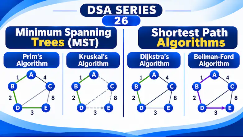
1. Introduction
Graphs are used to represent connections between objects, such as cities connected by roads, computers connected through networks, and locations connected through transportation systems.
In the previous article, we learned how to traverse graphs using BFS and DFS. But sometimes, simply visiting vertices is not enough. We need to solve problems involving costs, distances, and efficiency.
Two important graph problems are:
- Minimum Spanning Tree (MST): Connecting all vertices with the minimum total edge weight.
- Shortest Path: Finding the path with the minimum total cost or distance between vertices.
Although both problems involve minimizing weights, they solve different problems.
2. Minimum Spanning Tree (MST)
A Spanning Tree is a subgraph of a connected, undirected graph that:
- Includes every vertex.
- Remains connected.
- Contains no cycles.
A Minimum Spanning Tree is a spanning tree whose total edge weight is as small as possible.
For a graph containing \(V\) vertices, a spanning tree always contains exactly:
\[
V-1
\]
edges.
Example
Suppose we need to connect five locations using roads. Each road has a construction cost.
Instead of building every possible road, we want to connect all locations while spending as little as possible.
The MST gives us a solution that connects every location without unnecessary cycles and with minimum total cost.
Applications include:
- Designing computer networks.
- Connecting cities with roads or cables.
- Electrical network design.
- Minimizing infrastructure construction costs.
Two popular algorithms for finding MSTs are Prim’s Algorithm and Kruskal’s Algorithm.
3. Prim’s Algorithm
Prim’s Algorithm builds a Minimum Spanning Tree by starting from any vertex and gradually expanding the tree.
At every step, it chooses the minimum-weight edge connecting a vertex already in the tree to a vertex outside the tree.
Working
- Choose any starting vertex.
- Find the smallest edge connecting the current tree to an unvisited vertex.
- Add that edge and vertex to the tree.
- Repeat until every vertex is included.
The algorithm never adds an edge that connects two vertices already inside the tree, preventing cycles.
Example
Suppose the graph contains these weighted edges:
| Edge | Weight |
|---|---|
| A–B | 1 |
| B–C | 2 |
| C–D | 3 |
| D–E | 1 |
| A–C | 4 |
| B–D | 5 |
| C–E | 8 |
Starting from A:
- Select A–B (1).
- Select B–C (2).
- Select C–D (3).
- Select D–E (1).
The resulting MST contains four edges.
Total cost:
\[
1+2+3+1=7
\]
Prim’s Algorithm (Pseudocode)
Prim(graph, start):

    add start to MST

    while MST does not contain all vertices:

        find the minimum-weight edge
        connecting MST to an outside vertex

        add that edge and vertex to MST
Using an adjacency list and a priority queue, Prim’s Algorithm can run in:
\[
O((V+E)\log V)
\]
4. Kruskal’s Algorithm
Kruskal’s Algorithm builds an MST by selecting edges in increasing order of weight.
Unlike Prim’s Algorithm, it does not grow from a single starting vertex. Instead, it considers the smallest edges across the entire graph.
Working
- Sort all edges by increasing weight.
- Select the smallest edge.
- If adding it does not create a cycle, include it in the MST.
- If it creates a cycle, skip it.
- Continue until (V-1) edges have been selected.
Example
Using the same graph:
| Edge | Weight |
|---|---|
| A–B | 1 |
| D–E | 1 |
| B–C | 2 |
| C–D | 3 |
| A–C | 4 |
| B–D | 5 |
| C–E | 8 |
Kruskal selects:
- A–B (1)
- D–E (1)
- B–C (2)
- C–D (3)
These edges connect all five vertices without forming a cycle.
Total cost:
\[
1+1+2+3=7
\]
Kruskal’s Algorithm (Pseudocode)
Kruskal(graph):

    sort all edges by increasing weight

    for each edge:

        if adding edge does not create a cycle:

            add edge to MST

        if MST contains V-1 edges:

            stop
To efficiently check whether an edge creates a cycle, Kruskal commonly uses a data structure called Disjoint Set Union (DSU), also known as Union-Find. We will study this data structure separately when needed.
Its typical time complexity is:
\[
O(E\log E)
\]
because sorting the edges is the dominant operation.
5. Prim vs. Kruskal
| Feature | Prim | Kruskal |
|---|---|---|
| Approach | Grows one tree | Builds and merges components |
| Selection | Cheapest edge connecting tree to outside | Cheapest edge globally |
| Starting vertex | Required | Not required |
| Common data structure | Priority Queue | DSU / Union-Find |
| Time complexity | \(O((V+E)\log V)\) | \(O(E\log E)\) |
Both algorithms produce a Minimum Spanning Tree for a connected, weighted, undirected graph.
6. Shortest Path Problem
The Shortest Path Problem finds a path between vertices such that the sum of the edge weights along that path is minimum.
Unlike MST, we may be interested in the shortest route between a particular pair of vertices or from one starting vertex to all other vertices.
Example
Suppose we want to travel from A to E.
Possible routes include:
- A → B → C → E
- A → B → C → D → E
- A → C → E
Each route has a different total distance.
The shortest path algorithm determines which route has the smallest total weight.
Shortest path algorithms are useful in:
- GPS navigation.
- Network routing.
- Transportation systems.
- Robotics.
- Game pathfinding.
7. Dijkstra’s Algorithm
Dijkstra’s Algorithm finds the shortest paths from a starting vertex to all other reachable vertices in a weighted graph with non-negative edge weights.
It works by repeatedly selecting the unvisited vertex with the smallest known distance from the source and updating the distances of its neighbors.
This updating process is called relaxation.
Understanding Relaxation
Suppose the current shortest known distance from A to B is 5, and we discover another route through C:
A → C → B
If the distance from A to C is 2 and C to B is 1, then the new route costs:
\[
2+1=3
\]
Since 3 is smaller than 5, we update the distance to B.
This is relaxation: replacing a known distance with a smaller one when a better route is found.
Working of Dijkstra’s Algorithm
- Set the distance to the starting vertex as 0.
- Set all other distances to infinity.
- Select the unvisited vertex with the smallest known distance.
- Update the distances of its neighbors if a shorter route is found.
- Mark the selected vertex as visited.
- Repeat until all reachable vertices are processed.
Example
Using the same weighted graph, start at A.
| Vertex | Shortest distance from A |
|---|---|
| A | 0 |
| B | 1 |
| C | 3 |
| D | 6 |
| E | 7 |
The shortest path from A to E is:
A → B → C → D → E
Total distance:
\[
1+2+3+1=7
\]
Dijkstra’s Algorithm can efficiently solve this problem using a priority queue.
With an adjacency list and a binary heap:
\[
O((V+E)\log V)
\]
Important: Dijkstra’s Algorithm does not work correctly with negative edge weights. For graphs containing negative weights, another algorithm such as Bellman-Ford may be needed.
8. Bellman-Ford Algorithm
Bellman-Ford is another shortest path algorithm that can handle negative edge weights, provided the graph does not contain a reachable negative-weight cycle.
A negative-weight cycle is a cycle whose total edge weight is negative. Repeatedly traversing such a cycle can keep reducing the path cost, meaning a finite shortest path may not exist.
Working
- Set the source distance to 0 and all others to infinity.
- Relax all edges repeatedly.
- Repeat this process (V-1) times.
- Perform one additional pass to check for a reachable negative-weight cycle.
Why (V-1) iterations?
A shortest simple path in a graph with (V) vertices can contain at most (V-1) edges. Therefore, after (V-1) passes, all shortest paths should have been found if no negative cycle exists.
Time Complexity
\[
O(VE)
\]
Bellman-Ford is slower than Dijkstra in many common cases, but it supports negative edge weights and can detect negative-weight cycles.
9. Comparing Graph Algorithms
| Algorithm | Purpose | Important condition |
|---|---|---|
| Prim | Minimum Spanning Tree | Connected, undirected weighted graph |
| Kruskal | Minimum Spanning Tree | Connected, undirected weighted graph |
| Dijkstra | Shortest paths | Non-negative edge weights |
| Bellman-Ford | Shortest paths | Can handle negative weights; no reachable negative cycle |
Remember:
- MST minimizes the total weight required to connect all vertices.
- Shortest Path minimizes the distance between specified vertices or from a source to others.
These are different optimization problems, even though both use weighted graphs.
Minimum Spanning Trees and Shortest Path Algorithms are two important applications of graph theory.
Prim and Kruskal minimize the total cost of connecting all vertices. Dijkstra finds shortest paths when edge weights are non-negative, while Bellman-Ford can also handle negative weights.
Choosing the correct algorithm depends on the problem: whether we need to connect everything as cheaply as possible or find the cheapest route between locations.
In the next article, we will explore Eulerian Tours and Hamiltonian Tours, which focus on traversing edges and visiting vertices under specific conditions.
Originally published at farhanpaal.com — https://farhanpaal.com/articles/minimum-spanning-trees-and-shortest-path-algorithms/
Keep a copy
Read offline as a printout or PDF.
farhanpaal.comKeep reading

Strings: Understanding String Data
Learn how strings work in C, including character storage, null termination, indexing, traversal, and common string functions with simple examples.
Heaps: Representation and Implementation of Priority Queues
Learn how Min Heaps and Max Heaps work, how Binary Heaps are represented using arrays, and how insertion and deletion maintain the…

Recursion: Understanding the Basics
Understand recursion, base cases, recursive calls, and the call stack. Learn how to trace recursive functions and calculate factorial using simple C…