 Farhan Paal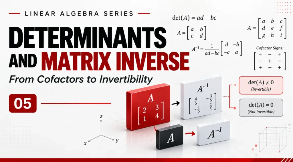
In the previous article, we learned how systems of linear equations can be represented using matrices and how Gaussian elimination and row reduction can be used to solve them.
We saw how a system such as:
\(x+y=7\)
\(2x+y=11\)
can be represented compactly as:
\[
A\mathbf{x}=\mathbf{b}
\]
We then used elementary row operations to simplify the system and eventually find the values of the unknown variables.
In this article, we will take our understanding of matrices one step further.
We will study two closely connected ideas: determinants and matrix inverses.
A determinant gives us important information about a square matrix. It can help us determine whether a matrix is invertible and whether a corresponding square system has a unique solution.
We will begin with the determinant of a \(2\times2\) matrix and gradually move toward larger matrices using minors, cofactors, and cofactor expansion.
Then we will use the determinant to understand invertibility.
Finally, we will study the matrix inverse itself: what it means, how it works, how to find the inverse of a 2×22\times2 matrix, and how row reduction can be used to find inverses of larger matrices.
The overall connection is:
\[
\text{Determinant}\rightarrow\text{Invertibility}\rightarrow\text{Matrix Inverse}
\]
1. What Is a Determinant?
A determinant is a single number associated with a square matrix.
For a matrix \(A\), the determinant is written as:
\[
\det(A)
\]
For a \(2\times2\) matrix:
\[
A=
\begin{bmatrix}
a&b\\
c&d
\end{bmatrix}
\]
the determinant is:
\[
\det(A)=ad-bc
\]
So a matrix containing four numbers gives us one number called its determinant.
For example:
\[
A=
\begin{bmatrix}
2&3\\
4&5
\end{bmatrix}
\]
Its determinant is:
\[
\det(A)=(2)(5)-(3)(4)
\]
Therefore:
\[
\det(A)=10-12
\]
So:
\[
\det(A)=-2
\]
The determinant of \(A\) is \(-2\).
2. Why Do Determinants Matter?
At first, the determinant may seem like just another calculation.
But it provides important information about a matrix.
One of its most important uses is determining whether a square matrix is invertible.
If:
\[
\det(A)\neq0
\]
then \(A\) is invertible.
If:
\[
\det(A)=0
\]
then \(A\) is not invertible.
This distinction becomes important when we study matrix inverses.
The determinant is also connected to:
- systems of linear equations
- matrix inverses
- linear transformations
- area and volume
- geometry
- numerical methods
- computer graphics
- scientific computing
So the determinant is not simply a formula to memorize.
It tells us something about the structure and behavior of a matrix.
3. Determinant of a \(2\times2\) Matrix
Let’s look more closely at the simplest case.
Consider:
\[
A=
\begin{bmatrix}
a&b\\
c&d
\end{bmatrix}
\]
The determinant is:
\[
\det(A)=ad-bc
\]
This is often called the \(ad-bc\) rule.
We multiply the entries on one diagonal:
\[
ad
\]
Then multiply the entries on the other diagonal:
\[
bc
\]
Finally, subtract:
\[
ad-bc
\]
For example:
\[
A=
\begin{bmatrix}
3&2\\
1&4
\end{bmatrix}
\]
Then:
\[
\det(A)=(3)(4)-(2)(1)
\]
Therefore:
\[
\det(A)=12-2
\]
So:
\[
\det(A)=10
\]
4. Understanding the ad−bcad-bc Rule
It is useful to understand the structure of the formula instead of simply memorizing it.
Start with:
\[
\begin{bmatrix}
a&b\\
c&d
\end{bmatrix}
\]
The two products are:
\[
ad
\]
and:
\[
bc
\]
The determinant is:
\[
ad-bc
\]
For example:
\[
\begin{bmatrix}
2&5\\
3&7
\end{bmatrix}
\]
The first diagonal product is:
\[
(2)(7)=14
\]
The second diagonal product is:
\[
(5)(3)=15
\]
Therefore:
\[
\det(A)=14-15
\]
So:
\[
\det(A)=-1
\]
The order matters.
The rule is:
\[
ad-bc
\]
not:
\[
bc-ad
\]
5. Determinant of a \(3\times3\) Matrix
The 2×22\times2 determinant is relatively simple.
But what happens when the matrix becomes larger?
Consider:
\[
A=
\begin{bmatrix}
a&b&c\\
d&e&f\\
g&h&i
\end{bmatrix}
\]
We now need a systematic way to calculate the determinant.
One important method is cofactor expansion.
Before we can understand cofactor expansion, however, we need to understand two related ideas:
- minors
- cofactors
These ideas allow us to break a larger determinant into smaller determinants.
6. What Is a Minor?
A minor is obtained by removing one row and one column from a matrix and then calculating the determinant of the remaining matrix.
Consider:
\[
A=
\begin{bmatrix}
a&b&c\\
d&e&f\\
g&h&i
\end{bmatrix}
\]
Suppose we want the minor corresponding to the element \(a\).
The element \(a\) is in row 1 and column 1.
Remove row 1 and column 1.
We are left with:
\[
\begin{bmatrix}
e&f\\
h&i
\end{bmatrix}
\]
The determinant of this smaller matrix is:
\[
ei-fh
\]
Therefore:
\[
M_{11}=ei-fh
\]
The subscripts tell us the position of the original element.
The first subscript represents the row, and the second represents the column.
7. Another Example of a Minor
Consider:
\[
A=
\begin{bmatrix}
1&2&3\\
4&5&6\\
7&8&9
\end{bmatrix}
\]
Suppose we want \(M_{12}\).
The element in row 1, column 2 is:
\(2\)
Remove row 1 and column 2.
The remaining matrix is:
\[
\begin{bmatrix}
4&6\\
7&9
\end{bmatrix}
\]
Its determinant is:
\[
M_{12}=(4)(9)-(6)(7)
\]
Therefore:
\[
M_{12}=36-42
\]
So:
\[
M_{12}=-6
\]
The general process is simple:
Choose an element → remove its row and column → calculate the determinant of the remaining matrix.
That determinant is the minor.
8. What Is a Cofactor?
A cofactor is closely related to a minor.
The cofactor \(C_{ij}\) is defined as:
\[
C_{ij}=(-1)^{i+j}M_{ij}
\]
This creates a specific pattern of positive and negative signs.
For a \(3\times3\) matrix, the pattern is:
\[
\begin{bmatrix}
+&-&+\\
-&+&-\\
+&-&+
\end{bmatrix}
\]
This sign pattern is essential when performing cofactor expansion.
9. The \(+,-,+\) Sign Pattern
Let’s understand why the signs alternate.
The cofactor formula is:
\[
C_{ij}=(-1)^{i+j}M_{ij}
\]
For the element in position \((1,1)\):
\[
(-1)^{1+1}=(-1)^2=+
\]
For position \((1,2)\):
\[
(-1)^{1+2}=(-1)^3=-
\]
For position \((1,3)\):
\[
(-1)^{1+3}=(-1)^4=+
\]
So the first row becomes:
\[
+,-,+
\]
Continuing the same pattern gives:
\[
\begin{bmatrix}
+&-&+\\
-&+&-\\
+&-&+
\end{bmatrix}
\]
A simple way to remember it is:
Start with \(+\) and alternate the signs across each row and column.
10. Minor vs Cofactor
It is important to distinguish a minor from a cofactor.
A minor is the determinant obtained after removing a particular row and column.
A cofactor is that minor multiplied by its corresponding sign.
In mathematical form:
\[
C_{ij}=(-1)^{i+j}M_{ij}
\]
For example, suppose:
\[
M_{12}=-6
\]
The position \((1,2)\) has a negative sign.
Therefore:
\[
C_{12}=-(-6)
\]
So:
\[
C_{12}=6
\]
The minor is \(-6\), while the cofactor is \(6\).
11. Cofactor Expansion
Now we can use minors and cofactors to calculate a \(3\times3\) determinant.
Consider:
\[
A=
\begin{bmatrix}
a&b&c\\
d&e&f\\
g&h&i
\end{bmatrix}
\]
We can expand along the first row.
The determinant is:
\[
\det(A)=aC_{11}+bC_{12}+cC_{13}
\]
Because the cofactor signs are:
\[
+,-,+
\]
we can write this as:
\[
\det(A)=aM_{11}-bM_{12}+cM_{13}
\]
Now calculate each minor.
For \(M_{11}\):
\[
M_{11}=
\begin{vmatrix}
e&f\\
h&i
\end{vmatrix}
\]
Therefore:
\[
M_{11}=ei-fh
\]
For \(M_{12}\):
\[
M_{12}=
\begin{vmatrix}
d&f\\
g&i
\end{vmatrix}
\]
Therefore:
\[
M_{12}=di-fg
\]
For \(M_{13}\):
\[
M_{13}=
\begin{vmatrix}
d&e\\
g&h
\end{vmatrix}
\]
Therefore:
\[
M_{13}=dh-eg
\]
Putting everything together:
\[
\det(A)=a(ei-fh)-b(di-fg)+c(dh-eg)
\]
This gives us a systematic way to calculate the determinant of a \(3\times3\) matrix.
12. Complete 3×33\times3 Example
Let’s work through a complete example.
Consider:
\[
A=
\begin{bmatrix}
1&2&3\\
0&4&5\\
1&0&6
\end{bmatrix}
\]
We will expand along the first row.
Using the \(+,-,+\) sign pattern:
\[
\det(A)=1M_{11}-2M_{12}+3M_{13}
\]
First, calculate \(M_{11}\).
Remove row 1 and column 1:
\[
M_{11}=
\begin{vmatrix}
4&5\\
0&6
\end{vmatrix}
\]
Therefore:
\[
M_{11}=(4)(6)-(5)(0)
\]
So:
\[
M_{11}=24
\]
Now calculate \(M_{12}\).
Remove row 1 and column 2:
\[
M_{12}=
\begin{vmatrix}
0&5\\
1&6
\end{vmatrix}
\]
Therefore:
\[
M_{12}=(0)(6)-(5)(1)
\]
So:
\[
M_{12}=-5
\]
Finally, calculate \(M_{13}\).
Remove row 1 and column 3:
\[
M_{13}=
\begin{vmatrix}
0&4\\
1&0
\end{vmatrix}
\]
Therefore:
\[
M_{13}=(0)(0)-(4)(1)
\]
So:
\[
M_{13}=-4
\]
Now substitute:
\[
\det(A)=1(24)-2(-5)+3(-4)
\]
Therefore:
\[
\det(A)=24+10-12
\]
So:
\[
\det(A)=22
\]
The determinant is \(22\).
Since:
\[
22\neq0
\]
the matrix is invertible.
13. Expanding Along Different Rows and Columns
Cofactor expansion does not have to be performed along the first row.
We can expand along any row or any column.
For example, we can expand along:
- the first row
- the second row
- the third row
- the first column
- the second column
- the third column
The final determinant will be the same.
However, some choices make the calculation much easier.
Consider:
\[
A=
\begin{bmatrix}
1&0&0\\
2&3&4\\
5&6&7
\end{bmatrix}
\]
The first row contains two zeros.
If we expand along the first row:
\[
\det(A)=1C_{11}+0C_{12}+0C_{13}
\]
Therefore:
\[
\det(A)=C_{11}
\]
We only need to calculate one \(2\times2\) determinant.
So when using cofactor expansion, look for a row or column containing zeros whenever possible.
14. Determinants and Row Operations
In the previous article, we learned about three elementary row operations:
- Swapping two rows
- Multiplying a row by a non-zero number
- Adding a multiple of one row to another
These operations have predictable effects on determinants.
Swapping two rows
When two rows are swapped, the determinant changes sign.
If:
\[
\det(A)=5
\]
then after swapping two rows:
\[
\det(A)=-5
\]
Multiplying a row by a number
If one row is multiplied by \(k\), the determinant is also multiplied by \(k\).
For example, if:
\[
\det(A)=4
\]
and one row is multiplied by \(3\), the new determinant is:
\[
12
\]
Adding a multiple of one row to another
If we perform:
\[
R_2\rightarrow R_2+3R_1
\]
the determinant remains unchanged.
These properties become particularly useful when we combine determinants with row reduction.
15. Determinant Through Row Reduction
We can also calculate determinants by using row operations to simplify a matrix.
Consider an upper triangular matrix:
\[
A=
\begin{bmatrix}
a&*&*\\
0&b&*\\
0&0&c
\end{bmatrix}
\]
For a triangular matrix, the determinant is simply the product of the diagonal entries:
\[
\det(A)=abc
\]
This means that if we can use row operations to transform a matrix into triangular form, calculating its determinant can become much easier.
However, we must carefully track any row swaps or row scaling because they change the determinant.
This creates an important connection between the two topics we have studied:
Gaussian elimination simplifies the matrix, while determinant rules tell us how those row operations affect the determinant.
16. Determinants and Invertibility
Now we reach one of the most important connections in this article.
For a square matrix \(A\):
\[
\det(A)\neq0
\]
means that \(A\) is **invertible**.
If:
\[
\det(A)=0
\]
then \(A\) is **singular**, meaning that it does not have an inverse.
Let’s see this with an example.
Consider:
\[
A=
\begin{bmatrix}
2&3\\
1&4
\end{bmatrix}
\]
Its determinant is:
\[
\det(A)=(2)(4)-(3)(1)
\]
Therefore:
\[
\det(A)=5
\]
Since:
\[
5\neq0
\]
the matrix is invertible.
Now consider:
\[
B=
\begin{bmatrix}
1&2\\
2&4
\end{bmatrix}
\]
Its determinant is:
\[
\det(B)=(1)(4)-(2)(2)
\]
Therefore:
\[
\det(B)=0
\]
So \(B\) is not invertible.
Notice that the second row is twice the first row:
\[
[2,4]=2[1,2]
\]
The rows do not contain independent information.
This is closely connected to the determinant being zero.
17. What Is a Matrix Inverse?
Now we can move to the second major idea of this article: the matrix inverse.
You may already be familiar with the inverse of an ordinary number.
For example, the reciprocal of \(5\) is:
\[
\frac{1}{5}
\]
because:
\[
5\times\frac{1}{5}=1
\]
The number \(1\) acts as the multiplicative identity.
Matrices have a similar concept.
For a square matrix \(A\), its inverse is written as:
\[
A^{-1}
\]
If the inverse exists, it satisfies:
\[
AA^{-1}=I
\]
and:
\[
A^{-1}A=I
\]
where \(I\) is the identity matrix.
The inverse essentially undoes the effect of the original matrix.
18. The Identity Matrix
Before going further, we need to understand the identity matrix.
For a \(2\times2\) matrix, the identity matrix is:
\[
I=
\begin{bmatrix}
1&0\\
0&1
\end{bmatrix}
\]
It behaves like the number \(1\) in ordinary multiplication.
For example:
\[
5\times1=5
\]
Similarly:
\[
AI=A
\]
and:
\[
IA=A
\]
for a compatible square matrix \(A\).
For a \(3\times3\) matrix, the identity matrix is:
\[
I=
\begin{bmatrix}
1&0&0\\
0&1&0\\
0&0&1
\end{bmatrix}
\]
The pattern is always the same:
ones on the main diagonal and zeros everywhere else.
19. How Does a Matrix Inverse Work?
Suppose:
\[
A=
\begin{bmatrix}
a&b\\
c&d
\end{bmatrix}
\]
and \(A^{-1}\) exists.
The inverse is the matrix that brings us back to the identity:
\[
AA^{-1}=I
\]
This is similar to ordinary numbers.
For example:
\[
5\times\frac{1}{5}=1
\]
For matrices:
\[
AA^{-1}=I
\]
The inverse can therefore be thought of as the matrix equivalent of a reciprocal.
There is, however, an important difference.
**Not every square matrix has an inverse.**
A matrix is invertible only when:
\[
\det(A)\neq0
\]
This is why the determinant we studied earlier is so important.
20. Finding the Inverse of a 2×22\times2 Matrix
For a \(2\times2\) matrix:
\[
A=
\begin{bmatrix}
a&b\\
c&d
\end{bmatrix}
\]
the inverse, when it exists, is:
\[
A^{-1}=
\frac{1}{ad-bc}
\begin{bmatrix}
d&-b\\
-c&a
\end{bmatrix}
\]
Notice that the denominator is exactly the determinant:
\[
ad-bc=\det(A)
\]
This is another reason the determinant matters.
The formula only works when:
\[
ad-bc\neq0
\]
because division by zero is undefined.
21. Complete \(2\times2\) Inverse Example
Consider:
\[
A=
\begin{bmatrix}
2&3\\
1&4
\end{bmatrix}
\]
First calculate the determinant:
\[
\det(A)=(2)(4)-(3)(1)
\]
Therefore:
\[
\det(A)=5
\]
Since:
\[
5\neq0
\]
the matrix has an inverse.
Using the inverse formula:
\[
A^{-1}
=
\frac{1}{5}
\begin{bmatrix}
4&-3\\
-1&2
\end{bmatrix}
\]
Therefore:
\[
A^{-1}
=
\begin{bmatrix}
\frac45&-\frac35\\
-\frac15&\frac25
\end{bmatrix}
\]
We can verify the result by multiplying \(A\) by \(A^{-1}\).
\[
AA^{-1}
=
\begin{bmatrix}
2&3\\
1&4
\end{bmatrix}
\begin{bmatrix}
\frac45&-\frac35\\
-\frac15&\frac25
\end{bmatrix}
\]
The result is:
\[
AA^{-1}
=
\begin{bmatrix}
1&0\\
0&1
\end{bmatrix}
\]
which is the identity matrix.
Therefore, the inverse is correct.
22. Finding an Inverse Using Row Reduction
The \(2\times2\) formula is convenient, but what about larger matrices?
This is where row reduction becomes useful again.
Suppose we have a matrix \(A\).
We place the identity matrix beside it:
\[
[A\mid I]
\]
Our goal is to transform the left side into the identity matrix.
Symbolically:
\[
[A\mid I]\rightarrow[I\mid A^{-1}]
\]
The same elementary row operations are applied to both sides.
This method is powerful because it does not require us to memorize a separate formula for every matrix size.
23. Complete Inverse Using Row Reduction
Consider:
\[
A=
\begin{bmatrix}
1&2\\
3&4
\end{bmatrix}
\]
We begin with:
\[
[A\mid I]
=
\left[
\begin{array}{cc|cc}
1&2&1&0\\
3&4&0&1
\end{array}
\right]
\]
Our goal is to turn the left side into:
\[
\begin{bmatrix}
1&0\\
0&1
\end{bmatrix}
\]
First eliminate the \(3\) below the first pivot:
\[
R_2\rightarrow R_2-3R_1
\]
This gives:
\[
\left[
\begin{array}{cc|cc}
1&2&1&0\\
0&-2&-3&1
\end{array}
\right]
\]
Now make the second pivot equal to \(1\):
\[
R_2\rightarrow-\frac12R_2
\]
We get:
\[
\left[
\begin{array}{cc|cc}
1&2&1&0\\
0&1&\frac32&-\frac12
\end{array}
\right]
\]
Now eliminate the \(2\) above the second pivot:
\[
R_1\rightarrow R_1-2R_2
\]
This gives:
\[
\left[
\begin{array}{cc|cc}
1&0&-2&1\\
0&1&\frac32&-\frac12
\end{array}
\right]
\]
The left side is now the identity matrix.
Therefore, the right side is the inverse:
\[
A^{-1}
=
\begin{bmatrix}
-2&1\\
\frac32&-\frac12
\end{bmatrix}
\]
This is the same idea as Gaussian elimination from the previous article, but now we are using it to transform a matrix into its inverse.
24. Checking a Matrix Inverse
Whenever we calculate an inverse, we can verify it.
Suppose we have:
\[
A^{-1}
\]
We can multiply:
\[
AA^{-1}
\]
If the result is:
\[
I
\]
then the inverse is correct.
We can also check:
\[
A^{-1}A=I
\]
For example, if:
\[
A=
\begin{bmatrix}
2&3\\
1&4
\end{bmatrix}
\]
and:
\[
A^{-1}
=
\begin{bmatrix}
\frac45&-\frac35\\
-\frac15&\frac25
\end{bmatrix}
\]
then:
\[
AA^{-1}=I
\]
This provides a direct way to verify our calculation.
25. When Does a Matrix Have No Inverse?
Not every square matrix is invertible.
The determinant gives us the condition:
\[
\det(A)=0
\]
If the determinant is zero, the matrix is singular and has no inverse.
For example:
\[
A=
\begin{bmatrix}
1&2\\
2&4
\end{bmatrix}
\]
Its determinant is:
\[
\det(A)=(1)(4)-(2)(2)
\]
Therefore:
\[
\det(A)=0
\]
So \(A^{-1}\) does not exist.
This is not an accident.
The rows are dependent:
\[
[2,4]=2[1,2]
\]
The matrix does not contain enough independent information to be reversed uniquely.
26. Determinants, Inverses, and Systems of Equations
Now we can connect everything we have learned.
A system of equations can be written as:
\[
A\mathbf{x}=\mathbf{b}
\]
If \(A\) is invertible, we can multiply both sides by \(A^{-1}\):
\[
A^{-1}A\mathbf{x}=A^{-1}\mathbf{b}
\]
Since:
\[
A^{-1}A=I
\]
we get:
\[
I\mathbf{x}=A^{-1}\mathbf{b}
\]
Therefore:
\[
\mathbf{x}=A^{-1}\mathbf{b}
\]
This gives us another way to think about solving a system.
In the previous article, we used **Gaussian elimination**.
Here, we can use the **matrix inverse**.
Both approaches are connected through the same underlying linear algebra.
For a square matrix:
\[
\det(A)\neq0
\]
means that \(A\) is invertible, and therefore the system has a unique solution.
27. Determinants and Matrix Inverse in Python
NumPy can calculate both determinants and matrix inverses.
For example:
import numpy as np

A = np.array([
    [2, 3],
    [1, 4]
])

det_A = np.linalg.det(A)
inverse_A = np.linalg.inv(A)

print("Determinant:")
print(det_A)

print("Inverse:")
print(inverse_A)
The determinant is:
55
and the inverse is:
[45−35−1525]\begin{bmatrix} \frac45&-\frac35\\ -\frac15&\frac25 \end{bmatrix}
In practical numerical computing, libraries such as NumPy perform these calculations efficiently.
However, understanding the mathematics behind the functions is still important.
28. Determinants and Matrix Inverse in Computer Science
Determinants and matrix inverses appear in many areas of computer science and applied mathematics.
Computer Graphics
Matrices are used for transformations such as rotation, scaling, and other geometric operations.
An inverse transformation can be used to reverse a transformation.
Computer Vision
Matrix operations are fundamental to representing geometric transformations and relationships between coordinate systems.
Scientific Computing
Systems of equations and matrix inverses appear throughout scientific and engineering calculations.
Statistics
Determinants appear in calculations involving covariance matrices and multivariate probability distributions.
Machine Learning
Linear algebra is used throughout machine learning, particularly when working with transformations, optimization, and statistical models.
In real applications, software libraries usually perform the numerical calculations.
The important thing is to understand the mathematical structure underneath those operations.
A Quick Summary
Let’s bring everything together.
- A determinant is a single number associated with a square matrix.
- For a 2×22\times2 matrix, the determinant follows the ad−bcad-bc rule.
- A 3×33\times3 determinant can be calculated using minors and cofactors.
- A minor is obtained by removing a row and column and calculating the determinant of the remaining matrix.
- A cofactor is a minor multiplied by its corresponding sign.
- Cofactor signs follow the pattern:
[+−+−+−+−+]\begin{bmatrix} +&-&+\\ -&+&-\\ +&-&+ \end{bmatrix}
- Determinants are affected predictably by elementary row operations.
- A square matrix with a non-zero determinant is invertible.
- A square matrix with determinant zero is singular and has no inverse.
- The identity matrix acts like 11 in matrix multiplication.
- The inverse of AA, written A−1A^{-1}, satisfies:
AA−1=A−1A=IAA^{-1}=A^{-1}A=I
- For a 2×22\times2 matrix, there is a direct formula for finding its inverse.
- Row reduction can also be used to find an inverse:
[A∣I]→[I∣A−1][A\mid I]\rightarrow[I\mid A^{-1}]
- If AA is invertible, a system:
Ax=bA\mathbf{x}=\mathbf{b}
can be solved using:
x=A−1b\mathbf{x}=A^{-1}\mathbf{b}
The Bigger Picture
In the previous article, we learned how matrices can represent and solve systems of linear equations.
We learned about augmented matrices, elementary row operations, Gaussian elimination, row echelon form, reduced row echelon form, and back substitution.
Now we have added another layer to our understanding.
We learned that a matrix has a property called the determinant.
The determinant can tell us whether a square matrix is invertible.
We then used that idea to understand the matrix inverse.
The connection can now be seen clearly:
Matrix→Determinant→Invertibility→Inverse\text{Matrix} \rightarrow \text{Determinant} \rightarrow \text{Invertibility} \rightarrow \text{Inverse}
We also saw that row reduction is useful in both solving systems and finding matrix inverses.
But matrices are not only useful for solving equations.
We can also use them to describe collections of vectors, combinations of vectors, and the spaces those vectors create.
In the next article, we will move from individual matrices and equations to a broader mathematical idea:
vector spaces, linear combinations, and span.
This will help us understand how vectors are organized and how more advanced concepts such as basis, dimension, linear independence, and rank emerge from them.