
Growth of Functions and Asymptotic Notations (Big-O, Big-Ω, Big-Θ)
Understand how functions grow as input size increases and learn Big-O, Big-Ω, and Big-Θ notation to compare algorithm efficiency.

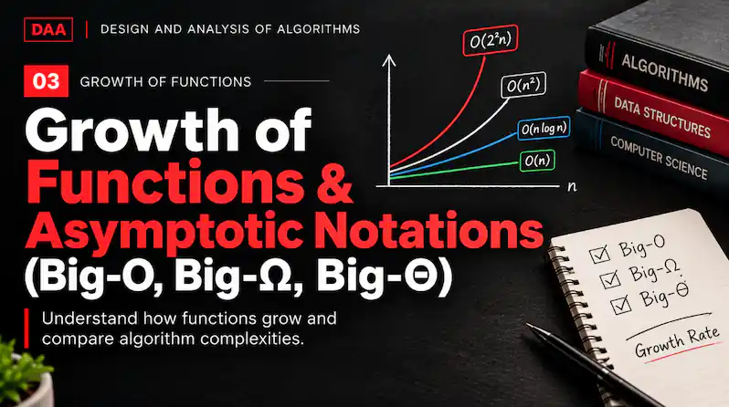
1. Introduction
When analyzing algorithms, we often want to know how their computational work grows as the input size increases.
For example, consider two algorithms:
- Algorithm A performs approximately \(n\) operations.
- Algorithm B performs approximately \(n^2\) operations.
For small inputs, their performance may appear similar. But as the input grows, Algorithm B requires significantly more work.
To compare algorithms mathematically, we study the growth of functions and use asymptotic notations such as Big-O, Big-Ω, and Big-Θ.
2. What Is Growth of Functions?
Growth of functions describes how a function’s value increases as its input becomes larger.
In algorithm analysis, these functions represent the amount of computational work performed by an algorithm.
Consider these functions:
\[
f(n)=n
\]
\[
g(n)=n^2
\]
\[
h(n)=2^n
\]
Their growth rates are different.
| Input (n) | (n) | (n^2) | (2^n) |
|---|---|---|---|
| 5 | 5 | 25 | 32 |
| 10 | 10 | 100 | 1,024 |
| 20 | 20 | 400 | 1,048,576 |
As the input increases, the exponential function \(2^n\) grows much faster than \(n\) or \(n^2\).
This helps us understand why some algorithms remain practical for large inputs while others become extremely slow.
3. Comparing Growth Rates
Some commonly encountered growth rates in algorithm analysis are:
| Complexity | Name | Growth |
|---|---|---|
| (O(1)) | Constant | Does not grow with input size |
| (O(\log n)) | Logarithmic | Grows slowly |
| (O(n)) | Linear | Proportional to input size |
| (O(n\log n)) | Linearithmic | Faster growth than linear |
| (O(n^2)) | Quadratic | Proportional to the square of input size |
| (O(n^3)) | Cubic | Proportional to the cube of input size |
| (O(2^n)) | Exponential | Grows extremely rapidly |
| (O(n!)) | Factorial | Extremely rapid growth |
These are common growth patterns. The actual complexity of an algorithm depends on the mathematical function describing its work.
4. Why Asymptotic Notations?
Suppose an algorithm performs:
\[
f(n)=3n^2+5n+2
\]
As the input size becomes very large, the \(n^2\) term dominates the other terms.
For example, when \(n=100\):
\[
3n^2=30,000
\]
\[
5n=500
\]
\[
2=2
\]
The quadratic term contributes most of the computational work.
Therefore, when analyzing large inputs, we focus on the dominant growth term and ignore constant factors and smaller-order terms.
This is the idea behind asymptotic analysis.
The three fundamental notations are:
- Big-O: Upper bound
- Big-Ω: Lower bound
- Big-Θ: Tight bound
5. Big-O Notation ( Upper Bound)
Big-O notation describes an upper bound on the growth of a function.
It tells us that a function does not grow faster than a particular rate, up to a constant factor, for sufficiently large input sizes.
Mathematically, \(f(n)=O(g(n))\) if there exist positive constants \(c\) and \(n_0\) such that:
\[
0\leq f(n)\leq c,g(n)
\]
for every \(n\geq n_0\).
Here:
- \(c\) is a positive constant.
- \(n_0\) is the starting input size from which the bound holds.
- \(g(n)\) is the function that provides the upper bound.
Example
Consider:
\[
f(n)=3n^2+5n+2
\]
We can show that:
\[
f(n)=O(n^2)
\]
For \(n\geq1\):
\[
3n^2+5n+2\leq10n^2
\]
Therefore, choosing \(c=10\) and \(n_0=1\) satisfies the Big-O definition.
So:
\[
\boxed{f(n)=O(n^2)}
\]
Big-O is commonly used to describe the worst-case growth of an algorithm, although mathematically it can describe an upper bound on any case or function.
6. Big-Ω Notation (Lower Bound)
Big-Ω notation describes a lower bound on the growth of a function.
It tells us that a function grows at least as fast as a particular rate, up to a constant factor, for sufficiently large input sizes.
Mathematically, \(f(n)=\Omega(g(n))\) if there exist positive constants \(c\) and \(n_0\) such that:
\[
0\leq c,g(n)\leq f(n)
\]
for every \(n\geq n_0\).
Example
Consider the same function:
\[
f(n)=3n^2+5n+2
\]
For \(n\geq1\):
\[
3n^2\leq3n^2+5n+2
\]
Therefore:
\[
\boxed{f(n)=\Omega(n^2)}
\]
The function grows at least as fast as \(n^2\), up to a constant factor.
7. Big-Θ Notation (Tight Bound)
Big-Θ notation describes a tight asymptotic bound.
It means that a function is bounded both above and below by the same growth rate, up to constant factors.
Mathematically, \(f(n)=\Theta(g(n))\) if there exist positive constants \(c_1,c_2\), and \(n_0\) such that:
\[
0\leq c_1g(n)\leq f(n)\leq c_2g(n)
\]
for every \(n\geq n_0\).
Example
Again:
\[
f(n)=3n^2+5n+2
\]
For \(n\geq1\):
\[
3n^2\leq f(n)\leq10n^2
\]
Therefore, the function is bounded both above and below by constant multiples of (n^2).
Hence:
\[
\boxed{f(n)=\Theta(n^2)}
\]
This means the function grows at the same asymptotic rate as (n^2).
8. Big-O vs. Big-Ω vs. Big-Θ
| Notation | Meaning | Describes |
|---|---|---|
| Big-O | Upper bound | Growth no faster than a specified rate |
| Big-Ω | Lower bound | Growth at least as fast as a specified rate |
| Big-Θ | Tight bound | Growth at the same asymptotic rate |
For example, if:
\[
f(n)=3n^2+5n+2
\]
Then all three statements are true:
\[
f(n)=O(n^2)
\]
\[
f(n)=\Omega(n^2)
\]
\[
f(n)=\Theta(n^2)
\]
The tightest description here is Θ((n^2)) because it captures both the upper and lower growth bounds.
9. Common Examples in Algorithms
Linear Search
In the worst case, linear search may examine every element of an array of size (n).
Therefore, its worst-case time complexity is:
\[
O(n)
\]
Since the worst-case number of comparisons is also proportional to (n), it can be described tightly as:
\[
\Theta(n)
\]
Binary Search
Binary Search repeatedly divides the search space approximately in half.
Its number of steps grows logarithmically:
\[
\Theta(\log n)
\]
Nested Loops
Consider two nested loops, each running (n) times.
The total number of iterations is:
\[
n\times n=n^2
\]
Therefore:
\[
\Theta(n^2)
\]
These examples show how asymptotic notation helps describe and compare algorithmic growth.
Conclusion
Growth of functions helps us understand how computational work increases as input size becomes larger.
Asymptotic notations allow us to describe this growth mathematically:
- Big-O describes an upper bound.
- Big-Ω describes a lower bound.
- Big-Θ describes a tight bound.
By focusing on dominant growth rates rather than exact operation counts, we can compare algorithms and understand their scalability.
In the next article, we will explore techniques for analyzing algorithm complexity, including the Substitution Method and Recursion Tree Method.
Quick quiz
5 questionsOriginally published at farhanpaal.com — https://farhanpaal.com/articles/growth-of-functions-and-asymptotic-notations-big-o-big-%cf%89-big-%ce%b8/
Keep a copy
Read offline as a printout or PDF.
farhanpaal.comKeep reading

Brute Force Strategy: When to Use It and Its Limitations
Understand the Brute Force strategy, its examples, advantages, limitations, time complexity, and when this straightforward approach is suitable.

What is DESIGN AND ANALYSIS OF ALGORITHM?
What is Design and Analysis of Algorithms (DAA)? Explore how algorithms are designed, analyzed for efficiency and correctness, and what this DAA…

Master Theorem: A Complete Guide
Learn the Master Theorem to solve recurrence relations quickly. Understand its three cases with step-by-step examples and complexity analysis.