
Merge Sort and Quick Sort: A Comparative Guide
Understand how Merge Sort and Quick Sort work with step-by-step examples, C implementations, and a comparison of their time and space complexity.

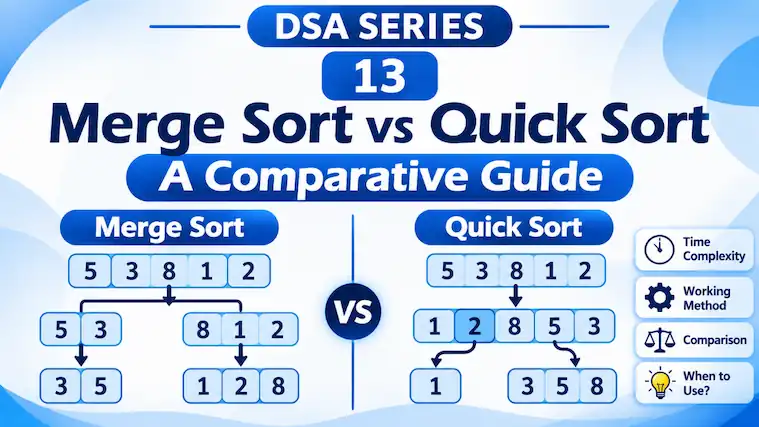
In the previous article, we learned three basic sorting algorithms: Bubble Sort, Selection Sort, and Insertion Sort.
Although these algorithms are useful for understanding sorting, they can become slow when working with large datasets.
Now let’s explore two more efficient sorting algorithms: Merge Sort and Quick Sort.
Both use a technique called <abbr title=”A problem-solving approach that divides a large problem into smaller parts, solves them, and combines the results.”>Divide and Conquer</abbr>. However, they approach sorting differently.
1. Merge Sort
Merge Sort works by repeatedly dividing an array into smaller parts until each part contains only one element. It then merges these parts back together in sorted order.
Let’s understand this with an example.
Consider:
int a[] = {5, 3, 8, 1, 2};Step 1: Divide the array into two halves.
             5   3   8   1   2
                  /   \
             5   3     8   1   2
Step 2: Continue dividing until each part contains one element.
            [5   3   8   1   2]
              /        \
           [5   3]     [8   1   2]
           /  \        /    \
         [5]   [3]    [8]   [1   2]
                             /   \
                           [1]    [2]
Now every part contains only one element. A single-element array is already sorted.
Step 3: Merge the elements in sorted order.
Compare 5 and 3. Since 3 is smaller, place it first.
Before:  [5]   [3]
After:    3     5
Now merge 1 and 2:
Before:  [1]   [2]
After:    1     2
We now have:
3 5 8 1 2Step 4: Merge the larger sorted portions.
Merge [3, 5] and [8].
Compare 3 and 8 → Take 3
Compare 5 and 8 → Take 5
Take the remaining 8

Result: 3   5   8
Merge [1, 2]:
Result: 1 2Step 5: Merge both sorted halves.
Now merge:
Left:   3   5   8
Right:  1   2
Compare the first available elements and take the smaller one each time:
Compare 3 and 1 → Take 1
Compare 3 and 2 → Take 2
Take the remaining 3, 5, 8
Final sorted array:
1 2 3 5 8That’s how Merge Sort works: divide the array into smaller parts and merge them back in sorted order.
C Implementation:
#include <stdio.h>

void merge(int a[], int left, int mid, int right) {
    int n1 = mid - left + 1;
    int n2 = right - mid;

    int L[n1], R[n2];

    for (int i = 0; i < n1; i++)
        L[i] = a[left + i];

    for (int j = 0; j < n2; j++)
        R[j] = a[mid + 1 + j];

    int i = 0, j = 0, k = left;

    while (i < n1 && j < n2) {
        if (L[i] <= R[j])
            a[k++] = L[i++];
        else
            a[k++] = R[j++];
    }

    while (i < n1)
        a[k++] = L[i++];

    while (j < n2)
        a[k++] = R[j++];
}

void mergeSort(int a[], int left, int right) {
    if (left < right) {
        int mid = left + (right - left) / 2;

        mergeSort(a, left, mid);
        mergeSort(a, mid + 1, right);

        merge(a, left, mid, right);
    }
}

int main() {
    int a[] = {5, 3, 8, 1, 2};
    int n = 5;

    mergeSort(a, 0, n - 1);

    for (int i = 0; i < n; i++)
        printf("%d ", a[i]);

    return 0;
}
Output:
1 2 3 5 8Notice that the function mergeSort() keeps dividing the array, while merge() combines the smaller sorted portions.
2. Quick Sort
Quick Sort also uses Divide and Conquer, but it works differently from Merge Sort.
Instead of dividing the array into equal halves, it selects one element as a pivot and rearranges the other elements around it.
A <abbr title=”An element selected to divide the array during Quick Sort.”>pivot</abbr> is the element used to partition the array into two groups:
- Elements smaller than or equal to the pivot.
- Elements greater than the pivot.
After partitioning, the pivot reaches its correct sorted position. We then apply the same process to the remaining groups.
Example:
Consider:
5 3 8 1 2Step 1: Select a pivot.
For this example, we’ll choose the last element, 2, as our pivot.
5 3 8 1 [2]Step 2: Place smaller elements before the pivot and larger elements after it.
Only 1 is smaller than 2.
We move 1 to the beginning and place the pivot immediately after it.
Before:  5   3   8   1   [2]

After:   1  [2]  8   5   3
The pivot 2 is now in its correct position.
Step 3: Apply Quick Sort to the remaining portions.
We now have:
1 | 2 | 8 5 3The left portion contains only one element, so it is already sorted.
For the right portion, select 3 as the pivot.
8 5 [3]Place the smaller elements before 3 and the larger elements after it.
Before:  8   5   [3]

After:  [3]  5   8
Now the complete array is:
1 2 3 5 8The array is sorted!
C Implementation:
#include <stdio.h>

void swap(int *a, int *b) {
    int temp = *a;
    *a = *b;
    *b = temp;
}

int partition(int a[], int low, int high) {
    int pivot = a[high];
    int i = low - 1;

    for (int j = low; j < high; j++) {
        if (a[j] <= pivot) {
            i++;
            swap(&a[i], &a[j]);
        }
    }

    swap(&a[i + 1], &a[high]);

    return i + 1;
}

void quickSort(int a[], int low, int high) {
    if (low < high) {
        int pi = partition(a, low, high);

        quickSort(a, low, pi - 1);
        quickSort(a, pi + 1, high);
    }
}

int main() {
    int a[] = {5, 3, 8, 1, 2};
    int n = 5;

    quickSort(a, 0, n - 1);

    for (int i = 0; i < n; i++)
        printf("%d ", a[i]);

    return 0;
}
Output:
1 2 3 5 8Here, partition() places the pivot in its correct position, while quickSort() repeats the process for the remaining portions.
3. Merge Sort vs. Quick Sort
Both algorithms are efficient, but their approaches and performance differ.
| Feature | Merge Sort | Quick Sort |
|---|---|---|
| Main idea | Divide into halves and merge | Partition around a pivot |
| Best-case time | O(n log n) | O(n log n) |
| Average-case time | O(n log n) | O(n log n) |
| Worst-case time | O(n log n) | O(n²) |
| Extra space | O(n) | O(log n) average |
| Stability | Stable | Usually unstable |
| Main operation | Merging | Partitioning |
Note: Quick Sort can require O(n) extra stack space in the worst case. Its performance depends heavily on pivot selection.
A <abbr title=”A sorting algorithm is stable if equal elements retain their original relative order after sorting.”>stable sorting algorithm</abbr> preserves the original order of elements that have equal values.
4. When Should We Use Them?
Merge Sort:
- When predictable O(n log n) performance is important.
- When working with linked lists or large datasets.
- When maintaining the original order of equal elements matters.
Its main disadvantage is that it requires additional memory for merging.
Quick Sort:
- When sorting arrays efficiently in practice.
- When additional memory usage should generally be kept low.
- When a good pivot-selection strategy is available.
Its disadvantage is that poor pivot selection can lead to O(n²) time complexity.
Merge Sort divides an array into smaller parts and merges them in sorted order, while Quick Sort selects a pivot and partitions the array around it.
Both are generally much more efficient than Bubble Sort, Selection Sort, and Insertion Sort for large datasets.
The main difference is that Merge Sort performs the major work while merging, whereas Quick Sort performs it while partitioning.
In the next article, we’ll compare different searching and sorting algorithms and understand when each one is most useful.
Further reading: Cornell University – Sorting Algorithms · Khan Academy – Merge Sort and Divide and Conquer · Carnegie Mellon University – Sorting Recitation Notes
Originally published at farhanpaal.com — https://farhanpaal.com/articles/merge-sort-and-quick-sort-a-comparative-guide/
Keep a copy
Read offline as a printout or PDF.
farhanpaal.comKeep reading

Space and Time Complexity in DSA
Understand time complexity, space complexity, Big O notation, and how to analyse algorithm efficiency with simple examples.

Types of Data Structures: A Complete Overview
Learn about the different types of data structures, including primitive, non-primitive, linear, non-linear, static, and dynamic structures, with simple examples and practical…
Circular Queues, Deques, and Priority Queues
Explore Circular Queues, Deques, and Priority Queues. Understand how they work, their operations, differences, and practical C implementations with simple examples.