
Articles / Linear Algebra · Part 7
Vector Spaces, Linear Combinations and Span Explained
Learn what vector spaces, linear combinations, and span mean in linear algebra, with clear examples, geometric explanations, and applications in AI.

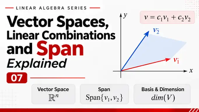
In linear algebra, we work with vectors and matrices to represent and solve mathematical problems. We have already learned how to perform operations on vectors, multiply matrices, solve systems of linear equations, and calculate matrix inverses.
But there is a deeper question:
What makes a collection of vectors mathematically meaningful, and how can we describe all the vectors that can be formed from a given collection?
To answer this, we need to understand three important concepts:
- Vector Spaces
- Linear Combinations
- Span
These concepts are fundamental to linear algebra. They help us understand how vectors relate to one another, how new vectors can be constructed, and what kinds of values or directions a collection of vectors can represent.
Let’s understand them step by step.
1. What Is a Vector Space?
A vector space is a collection of objects called vectors in which we can perform two operations:
- Vector addition
- Scalar multiplication
The results of these operations must remain within the same collection.
In simple terms, a vector space is a mathematical environment where vectors can be added together and multiplied by numbers while satisfying certain rules.
For example, consider vectors in two-dimensional space:
\( \mathbf{u} = (2,3) \)
\( \mathbf{v} = (4,1) \)
We can add them:
\[
\mathbf{u}+\mathbf{v}=(2,3)+(4,1)
=(6,4)
\]
We can also multiply a vector by a scalar:
\[
3\mathbf{u}=3(2,3)=(6,9)
\]
Both results are still vectors in two-dimensional space.
This is one of the important properties of a vector space: performing these operations does not take us outside the space.
However, a collection is not automatically a vector space just because its elements look like vectors. It must satisfy a set of mathematical rules.
The Properties of a Vector Space
A vector space over the real numbers must satisfy the following properties.
Let \(\mathbf{u}\), \(\mathbf{v}\), and \(\mathbf{w}\) be vectors, and let \(a\) and \(b\) be real numbers.
1. Closure under addition
Adding two vectors must produce another vector in the same space.
\[
\mathbf{u}+\mathbf{v}\in V
\]
2. Commutativity of addition
The order of vector addition does not matter.
\[
\mathbf{u}+\mathbf{v}=\mathbf{v}+\mathbf{u}
\]
3. Associativity of addition
The grouping of vector addition does not change the result.
\[
(\mathbf{u}+\mathbf{v})+\mathbf{w}
=\mathbf{u}+(\mathbf{v}+\mathbf{w})
\]
4. Existence of a zero vector
There must be a zero vector that does not change a vector when added to it.
\[
\mathbf{u}+\mathbf{0}=\mathbf{u}
\]
For example, in two-dimensional space, the zero vector is \((0,0)\).
5. Existence of an additive inverse
Every vector must have an opposite vector that produces the zero vector when added.
\[
\mathbf{u}+(-\mathbf{u})=\mathbf{0}
\]
For example:
\[
(2,3)+(-2,-3)=(0,0)
\]
6. Closure under scalar multiplication
Multiplying a vector by a real number must produce another vector in the same space.
\[
a\mathbf{u}\in V
\]
7. Associativity of scalar multiplication
Multiplying a vector by two scalars in sequence is equivalent to multiplying it by their product.
\[
a(b\mathbf{u})=(ab)\mathbf{u}
\]
8. Scalar identity
Multiplying a vector by 1 must leave it unchanged.
\[
1\mathbf{u}=\mathbf{u}
\]
9. Distributivity over vector addition
Multiplying a sum of vectors by a scalar is equivalent to multiplying each vector separately and then adding the results.
\[
a(\mathbf{u}+\mathbf{v})
=a\mathbf{u}+a\mathbf{v}
\]
10. Distributivity over scalar addition
Multiplying a vector by the sum of two scalars is equivalent to multiplying the vector by each scalar and adding the results.
\[
(a+b)\mathbf{u}=a\mathbf{u}+b\mathbf{u}
\]
All these properties together define a vector space.
Examples of Vector Spaces
Some common examples include:
- \(\mathbb{R}^2\): All ordered pairs of real numbers.
- \(\mathbb{R}^3\): All ordered triples of real numbers.
- \(\mathbb{R}^n\): All vectors containing n real components.
- Polynomial spaces: Collections of polynomials with real coefficients.
- Matrix spaces: Collections of matrices of a fixed size with real entries.
For example, the following vectors belong to \(\mathbb{R}^2\):
\[
(1,2),\quad (3,4),\quad (-2,5),\quad (0,0)
\]
Each vector has two real-number components.
Similarly, \(\mathbb{R}^3\) contains vectors with three components, such as:
\[
(2,4,1),\quad (0,3,5),\quad (1,1,1)
\]
Understanding Vector Spaces Geometrically
A vector space can also be understood through geometry.
- \(\mathbb{R}^2\) represents the entire two-dimensional plane.
- \(\mathbb{R}^3\) represents the entire three-dimensional space.
In \(\mathbb{R}^2\), we can move in any direction and reach any point in the plane using a suitable vector.
The important idea is that a vector space is not just a collection of individual vectors. It describes a complete mathematical structure in which vector addition and scalar multiplication are valid.
2. What Is a Linear Combination?
Now that we understand vector spaces, let’s look at how new vectors can be created from existing vectors.
A linear combination is an expression formed by multiplying vectors by scalars and then adding the results.
In simple terms, we take one or more vectors, multiply them by numbers, and add them together to create another vector.
Consider two vectors:
\[
\mathbf{v}_1=(1,2)
\]
\[
\mathbf{v}_2=(3,1)
\]
We can multiply the first vector by 2 and the second vector by 3:
\[
2\mathbf{v}_1=(2,4)
\]
\[
3\mathbf{v}_2=(9,3)
\]
Now add them:
\[
2\mathbf{v}_1+3\mathbf{v}_2
=(2,4)+(9,3)
=(11,7)
\]
Therefore, \((11,7)\) is a linear combination of the two original vectors.
General Formula
For a collection of vectors \(\mathbf{v}_1,\mathbf{v}_2,\ldots,\mathbf{v}_n\), a linear combination is written as:
\[
\mathbf{v}=c_1\mathbf{v}_1+c_2\mathbf{v}_2+\cdots+c_n\mathbf{v}_n
\]
Where:
- \(\mathbf{v}_1,\mathbf{v}_2,\ldots,\mathbf{v}_n\) are the given vectors.
- \(c_1,c_2,\ldots,c_n\) are scalars.
- \(\mathbf{v}\) is the resulting vector.
The scalars determine how much each vector contributes to the final result.
A Step-by-Step Example
Suppose we have:
\[
\mathbf{v}_1=(1,0),\qquad \mathbf{v}_2=(0,1)
\]
We want to construct the vector:
\(\mathbf{b}=(5,3)\)
Can we express it as a linear combination of these two vectors?
Let’s try:
\[
\mathbf{b}=5\mathbf{v}_1+3\mathbf{v}_2
\]
Substituting the vectors:
\[
=5(1,0)+3(0,1)
\]
\[
=(5,0)+(0,3)
\]
\[
=(5,3)
\]
Therefore:
\[
(5,3)=5(1,0)+3(0,1)
\]
We have successfully represented the target vector as a linear combination of the two given vectors.
Can Every Vector Be a Linear Combination?
Not necessarily.
It depends on the vectors we are given.
For example, suppose we only have:
\[
\mathbf{v}_1=(1,2)
\]
Any linear combination of this single vector has the form:
\[
c\mathbf{v}_1=c(1,2)=(c,2c)
\]
This means we can create vectors such as:
\[
(1,2),\quad (2,4),\quad (-3,-6),\quad (0,0)
\]
But we cannot create \((1,3)\), because there is no scalar \(c\) that simultaneously satisfies:
\(c=1\) and \(2c=3\).
Therefore, not every vector in \(\mathbb{R}^2\) can be constructed from this single vector.
This leads us to our next concept: span.
3. What Is Span?
The span of a collection of vectors is the set of all possible linear combinations of those vectors.
In other words, span describes every vector we can create using the given vectors by multiplying them by scalars and adding the results.
It tells us how much of a vector space a particular collection of vectors can cover.
General Definition
For vectors \(\mathbf{v}_1,\mathbf{v}_2,\ldots,\mathbf{v}_n\), their span is written as:
\[
\operatorname{Span}{\mathbf{v}_1,\mathbf{v}_2,\ldots,\mathbf{v}_n}
\]
It contains every vector of the form:
\[
c_1\mathbf{v}_1+c_2\mathbf{v}_2+\cdots+c_n\mathbf{v}_n
\]
where the coefficients can be any real numbers.
Example 1: The Span of One Vector
Consider:
\[
\mathbf{v}=(1,2)
\]
Its span is:
\[
\operatorname{Span}{(1,2)}
={c(1,2)\in\mathbb{R}}
\]
This produces vectors such as:
\[
(1,2),\quad (2,4),\quad (-1,-2),\quad (0,0)
\]
Geometrically, all these vectors lie on the same straight line passing through the origin.
Therefore, the span of a single nonzero vector in \(\mathbb{R}^2\) is a line through the origin.
Example 2: The Span of Two Vectors
Consider:
\[
\mathbf{v}_1=(1,0),\qquad \mathbf{v}_2=(0,1)
\]
Their span is:
\[
\operatorname{Span}{(1,0),(0,1)}
\]
A general linear combination is:
\[
a(1,0)+b(0,1)
\]
\[
=(a,0)+(0,b)
\]
\[
=(a,b)
\]
Since both \(a\) and \(b\) can be any real numbers, we can create every vector in \(\mathbb{R}^2\).
Therefore:
\[
\operatorname{Span}{(1,0),(0,1)}=\mathbb{R}^2
\]
These two vectors span the entire two-dimensional plane.
Example 3: When Two Vectors Span Only a Line
Consider:
\[
\mathbf{v}_1=(1,2),\qquad \mathbf{v}_2=(2,4)
\]
Notice that the second vector is simply twice the first:
\[
\mathbf{v}_2=2\mathbf{v}_1
\]
Any linear combination of these vectors becomes:
\[
a(1,2)+b(2,4)
\]
\[
=(a+2b,\ 2a+4b)
\]
Let \(c=a+2b\). Then:
\[
=(c,2c)
\]
Every resulting vector lies on the line \(y=2x\).
Therefore, although we have two vectors, they span only a line, not the entire plane.
This example shows that the number of vectors alone does not determine how much space they can cover.
Their directions and relationships also matter.
4. Geometric Interpretation of Span
Span becomes easier to understand when we visualize it geometrically.
Depending on the vectors and the space in which they exist, their span can represent different geometric structures.
Case 1: A Single Nonzero Vector
In \(\mathbb{R}^2\), a single nonzero vector spans a line passing through the origin.
<figure> <img src=”vector-span-line.png” alt=”A vector spanning a straight line through the origin” /> </figure>
Case 2: Two Non-Collinear Vectors in \(\mathbb{R}^2\)
If two vectors point in different directions and are not scalar multiples of each other, they span the entire two-dimensional plane.
For example:
\[
\mathbf{v}_1=(1,0),\qquad \mathbf{v}_2=(0,1)
\]
Together, they can create any vector in the plane.
Case 3: Two Collinear Vectors
If two nonzero vectors lie along the same line, one can be expressed as a scalar multiple of the other.
Their span is still only a line.
Case 4: Three Independent Vectors in \(\mathbb{R}^3\)
Three vectors that are not confined to the same plane and are linearly independent can span the entire three-dimensional space.
For example:
\[
(1,0,0),\quad (0,1,0),\quad (0,0,1)
\]
These vectors can create any vector in \(\mathbb{R}^3\).
The geometric interpretation helps us understand an important point: span describes the region or set of vectors that can be reached through linear combinations.
5. How Are Vector Spaces, Linear Combinations and Span Related?
These three concepts are closely connected, but they describe different things.
| Concept | Meaning |
|---|---|
| Vector Space | A mathematical structure in which vector addition and scalar multiplication satisfy specific rules. |
| Linear Combination | A method of creating a new vector by multiplying vectors by scalars and adding them. |
| Span | The complete set of all possible linear combinations of given vectors. |
Let’s connect them using a simple example.
Suppose we have two vectors:
\[
\mathbf{v}_1=(1,0),\qquad \mathbf{v}_2=(0,1)
\]
Step 1: Vector Space
Both vectors belong to \(\mathbb{R}^2\), which is a vector space.
Step 2: Linear Combination
We multiply them by arbitrary scalars and add them:
\[
a\mathbf{v}_1+b\mathbf{v}_2
\]
Step 3: Span
All possible results form:
\[
\operatorname{Span}{\mathbf{v}_1,\mathbf{v}_2}=\mathbb{R}^2
\]
So, a vector space provides the mathematical environment, a linear combination provides the method, and span describes all the possible results.
6. Why Are These Concepts Important in Computer Science and AI?
Vector spaces, linear combinations, and span are not just theoretical mathematical ideas. They are used throughout computer science, data science, machine learning, and artificial intelligence.
1. Machine Learning
Machine learning models often represent data as vectors.
For example, a dataset might represent each student using three features:
\[
\mathbf{x}=(\text{Study Hours},\text{Attendance},\text{Previous Score})
\]
A model can combine these features using weights:
\[
y=w_1x_1+w_2x_2+w_3x_3+b
\]
This is a linear combination of input features, with an additional bias term.
The weights determine how much each feature contributes to the model’s output.
2. Neural Networks
Neural networks perform many operations involving vectors and matrices.
A basic layer can be represented as:
\[
\mathbf{y}=W\mathbf{x}+\mathbf{b}
\]
Here:
- \(\mathbf{x}\) is the input vector.
- \(W\) is a weight matrix.
- \(\mathbf{b}\) is a bias vector.
- \(\mathbf{y}\) is the resulting vector before applying an activation function.
Matrix multiplication combines input values using weighted linear combinations.
Understanding vector spaces makes it easier to understand how these calculations work.
3. Data Representation
In data science, observations are frequently represented as points in a multidimensional vector space.
For example, an image can be represented using a large collection of pixel values, while a document can be represented using numerical features or embeddings.
These representations allow computers to perform mathematical operations on information.
4. Dimensionality Reduction
Techniques such as Principal Component Analysis (PCA) use linear algebra to represent data using fewer dimensions.
PCA identifies important directions in the data and projects observations onto a lower-dimensional space.
The concepts of vectors, span, and basis help explain how these transformations work.
5. Computer Graphics
Computer graphics uses vectors to represent positions, directions, and movements.
Operations involving vectors and matrices allow objects to be rotated, scaled, translated, and transformed in two-dimensional and three-dimensional environments.
7. Practical Example Using Python and NumPy
Let’s see how linear combinations and span can be explored programmatically.
Python’s NumPy library provides tools for working with vectors and matrices.
First, import NumPy:
import numpy as npCreate two vectors:
v1 = np.array([1, 0])
v2 = np.array([0, 1])
Now create a linear combination:
result = 5 * v1 + 3 * v2

print(result)
Output:
[5 3]We have created the vector \((5,3)\) using a linear combination of two vectors.
Checking Another Linear Combination
v1 = np.array([1, 2])
v2 = np.array([2, 4])

result = 3 * v1 - 2 * v2

print(result)
Output:
[-1 -2]Both vectors lie along the same line. Their linear combinations also remain on that line.
Using Matrix Rank to Understand Span
The rank of a matrix tells us the number of linearly independent columns or rows.
It can help us understand how many independent directions a collection of vectors provides.
A = np.array([
    [1, 2],
    [2, 4]
])

print(np.linalg.matrix_rank(A))
Output:
1The two columns are linearly dependent because the second column is twice the first.
Therefore, they provide only one independent direction.
Now consider:
B = np.array([
    [1, 0],
    [0, 1]
])

print(np.linalg.matrix_rank(B))
Output:
2The two columns are linearly independent and span the entire two-dimensional space.
We will explore rank and linear independence in greater detail in a later article.
8. Common Misconceptions
Before moving forward, let’s clarify a few common misunderstandings.
1. Every collection of vectors is a vector space.
Not necessarily. A collection must satisfy all the vector space properties, including closure under addition and scalar multiplication.
2. A linear combination always produces a new vector.
Not necessarily a different vector. Depending on the scalars, it may produce an existing vector or even the zero vector.
3. Two vectors always span a plane.
No. If the vectors are scalar multiples of each other, they span only a line.
4. Span and vector space mean the same thing.
They are related but different. A vector space is a mathematical structure, whereas the span of a collection is the set of all its possible linear combinations.
5. More vectors always mean a larger span.
Not necessarily. Adding a vector that is already a linear combination of the existing vectors does not expand the span.
9. Summary
In this article, we explored three fundamental concepts of linear algebra.
- Vector Spaces: Mathematical structures in which vector addition and scalar multiplication follow specific rules.
- Linear Combinations: Expressions formed by multiplying vectors by scalars and adding them together.
- Span: The set of all possible linear combinations of a given collection of vectors.
We also explored their geometric interpretations, practical examples, and applications in machine learning, neural networks, data science, and computer graphics.
The key idea is that vectors can be combined to create other vectors, and the span tells us exactly which vectors can be created from a given collection.
What’s Next?
Now that we understand vector spaces, linear combinations, and span, we can move toward another important question:
How do we determine whether a collection of vectors is independent, and what is the minimum number of vectors needed to describe a space?
This brings us to the next article:
Article 8: Basis, Dimension, Linear Independence and Rank Explained
These concepts will help us understand the structure of vector spaces more deeply and prepare us for eigenvalues, eigenvectors, and matrix factorization.
Originally published at farhanpaal.com — https://farhanpaal.com/articles/vector-spaces-linear-combinations-and-span-explained/
Keep a copy
Read offline as a printout or PDF.
farhanpaal.comKeep reading
Linear Algebra: The Conclusion | What You’ve Learned and Where to Go Next
A complete journey through Linear Algebra — revisit key concepts, understand how they connect, explore real-world applications, and discover what to learn…
Vector and Matrix Operations Explained: Dot Product, Matrix Multiplication, and Transpose
Learn the most important vector and matrix operations, including vector addition, dot products, matrix multiplication, and transpose, with practical examples.
Applications in Computer Science: Graphics, Neural Networks, SVD in Recommendation Systems, and Robotics
Explore how linear algebra powers computer graphics, neural networks, recommendation systems, robotics, and modern computer science.