
Articles / Linear Algebra · Part 6
Application: Solving Linear Systems Using Matrix Inverses
Learn how to solve systems of linear equations using matrix inverses, with step-by-step examples, determinant calculations, and practical Python applications.

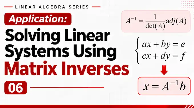
In the previous articles, we explored systems of linear equations, Gaussian elimination, determinants, and matrix inverses.
We learned how to represent a system of equations using matrices and how to determine whether a square matrix has an inverse.
But an important question remains:
How can we use a matrix inverse to solve a system of linear equations?
This is one of the most useful applications of matrix inverses in linear algebra.
Instead of solving equations individually, we can represent the entire system as a matrix equation and use the inverse to find the unknown values.
Let’s understand how this works, step by step.
1. Revisiting Systems of Linear Equations
A system of linear equations consists of two or more linear equations containing the same unknown variables.
For example:
\(2x+y=5\)
\(x+y=3\)
Our objective is to find the values of \(x\) and \(y\) that satisfy both equations simultaneously.
In this example:
\(x=2,\qquad y=1\)
satisfies both equations.
We can solve such systems using methods like substitution, elimination, and Gaussian elimination.
However, when dealing with larger systems, representing the equations in matrix form makes the calculations more organized.
2. Representing a System in Matrix Form
Consider the same system:
\(2x+y=5\)
\(x+y=3\)
We can separate its coefficients, variables, and constant values.
The coefficient matrix is:
\[
A=
\begin{bmatrix}
2&1\
1&1
\end{bmatrix}
\]
The variable matrix is:
\[
\mathbf{x}=
\begin{bmatrix}
x\
y
\end{bmatrix}
\]
The constant matrix is:
\[
\mathbf{b}=
\begin{bmatrix}
5\
3
\end{bmatrix}
\]
We can combine these matrices into one equation:
\(A\mathbf{x}=\mathbf{b}\)
This is the standard matrix representation of a system of linear equations.
Here:
- \(A\) represents the coefficients of the variables.
- \(\mathbf{x}\) represents the unknown variables.
- \(\mathbf{b}\) represents the constant values.
Instead of writing several equations separately, we can work with a single matrix equation.
3. Understanding the Main Idea
We have:
\(A\mathbf{x}=\mathbf{b}\)
Our objective is to isolate \(\mathbf{x}\).
In ordinary arithmetic, if:
\(2x=10\)
we divide both sides by 2:
\(x=\frac{10}{2}=5\)
In matrix mathematics, the equivalent operation is multiplication by the inverse matrix.
Recall from Article 5 that the inverse of a matrix \(A\) is written as \(A^{-1}\).
It satisfies:
\(A^{-1}A=I\)
where \(I\) is the identity matrix.
Therefore, if we multiply both sides of our matrix equation by \(A^{-1}\), we get:
\(A^{-1}A\mathbf{x}=A^{-1}\mathbf{b}\)
Since:
\(A^{-1}A=I\)
we obtain:
\(I\mathbf{x}=A^{-1}\mathbf{b}\)
And because multiplying a vector by the identity matrix does not change it:
\[\mathbf{x}=A^{-1}\mathbf{b}\]
This is the formula for solving a system of linear equations using a matrix inverse.
The central idea is simple:
If the coefficient matrix has an inverse, we can multiply the constant vector by that inverse to find the unknown variables.
4. A Complete Example: Solving a System Using the Inverse
Let’s solve the following system:
\(2x+y=5\)
\(x+y=3\)
We already know its matrix representation:
\[
A=
\begin{bmatrix}
2&1\
1&1
\end{bmatrix}
\]
\[
\mathbf{x}=
\begin{bmatrix}
x\
y
\end{bmatrix}
\]
\[
\mathbf{b}=
\begin{bmatrix}
5\
3
\end{bmatrix}
\]
Therefore:
\(A\mathbf{x}=\mathbf{b}\)
Our next step is to calculate the inverse of \(A\).
5. Step 1: Calculate the Determinant
Before calculating the inverse, we must check whether the matrix is invertible.
Recall the determinant formula for a \(2\times2\) matrix:
\(\det(A)=ad-bc\)
Our matrix is:
\[
A=
\begin{bmatrix}
2&1\
1&1
\end{bmatrix}
\]
Therefore:
\(\det(A)=(2\times1)-(1\times1)\)
\(\det(A)=2-1\)
\[\det(A)=1\]
Since the determinant is not zero, the matrix is invertible.
This means we can calculate its inverse and use it to solve the system.
6. Step 2: Calculate the Matrix Inverse
For a \(2\times2\) matrix:
\[
A=
\begin{bmatrix}
a&b\
c&d
\end{bmatrix}
\]
the inverse is:
\[
A^{-1}=
\frac{1}{ad-bc}
\begin{bmatrix}
d&-b\
-c&a
\end{bmatrix}
\]
Our matrix is:
\[
A=
\begin{bmatrix}
2&1\
1&1
\end{bmatrix}
\]
Substituting its values:
\[
A^{-1}=
\frac{1}{(2\times1)-(1\times1)}
\begin{bmatrix}
1&-1\
-1&2
\end{bmatrix}
\]
Since the determinant is 1:
\[
A^{-1}=
\begin{bmatrix}
1&-1\
-1&2
\end{bmatrix}
\]
We have now found the inverse of the coefficient matrix.
7. Step 3: Apply the Inverse Formula
Recall our main formula:
\(\mathbf{x}=A^{-1}\mathbf{b}\)
We have:
\[
A^{-1}=
\begin{bmatrix}
1&-1\
-1&2
\end{bmatrix}
\]
and:
\[
\mathbf{b}=
\begin{bmatrix}
5\
3
\end{bmatrix}
\]
Substituting:
\begin{bmatrix}
1&-1\
-1&2
\end{bmatrix}
\begin{bmatrix}
5\
3
\end{bmatrix}
\]
Now perform matrix multiplication.
For the first row:
\(x=(1\times5)+(-1\times3)\)
\(x=5-3=2\)
For the second row:
\(y=(-1\times5)+(2\times3)\)
\(y=-5+6=1\)
Therefore:
\(x=2,\qquad y=1\)
We have successfully solved the system using a matrix inverse.
8. Step 4: Verify the Answer
Whenever we solve a mathematical problem, it is important to verify our result.
We found:
\(x=2,\qquad y=1\)
Let’s substitute these values into the original equations.
First equation:
\(2x+y=5\)
\(2(2)+1=5\)
\(5=5\)
Second equation:
\(x+y=3\)
\(2+1=3\)
\(3=3\)
Both equations are satisfied.
Therefore, our solution is correct.
9. Why Does This Method Work?
The inverse method works because a matrix inverse reverses the effect of multiplying by the original matrix.
Consider:
\(A\mathbf{x}=\mathbf{b}\)
The matrix \(A\) transforms the unknown vector \(\mathbf{x}\) into the vector \(\mathbf{b}\).
When we multiply by \(A^{-1}\), we reverse that transformation:
\(A^{-1}(A\mathbf{x})=A^{-1}\mathbf{b}\)
The original vector is recovered:
\(\mathbf{x}=A^{-1}\mathbf{b}\)
This is similar to how division reverses multiplication in ordinary arithmetic.
However, remember that this method requires \(A\) to be a square, invertible matrix.
10. What Happens When a Matrix Is Not Invertible?
The inverse method cannot be applied when the coefficient matrix has no inverse.
For a square matrix:
\(\det(A)=0\)
means that the matrix is singular.
Consider:
\[
A=
\begin{bmatrix}
1&2\
2&4
\end{bmatrix}
\]
Its determinant is:
\(\det(A)=(1\times4)-(2\times2)\)
\(\det(A)=4-4=0\)
Therefore:
\(A^{-1}\text{ does not exist}\)
We cannot use:
\(\mathbf{x}=A^{-1}\mathbf{b}\)
for this matrix.
However, this does not automatically mean that the original system has no solution.
Depending on the constant vector, a singular system may have:
- No solution.
- Infinitely many solutions.
For example, consider:
\(x+2y=3\)
\(2x+4y=6\)
The second equation is simply twice the first equation.
Both equations describe the same line, so infinitely many pairs of values satisfy the system.
This is why understanding determinants and invertibility is important before applying the inverse method.
11. Solving Linear Systems Using Python and NumPy
So far, we have performed the calculations manually.
In practical applications, systems can contain hundreds or thousands of equations. Performing every matrix operation by hand would be extremely time-consuming.
Python libraries such as NumPy make these calculations easier.
Let’s solve our earlier example using Python.
import numpy as np

A = np.array([
    [2, 1],
    [1, 1]
])

b = np.array([5, 3])

# Calculate the determinant
det_A = np.linalg.det(A)

print("Determinant:")
print(det_A)

# Calculate the inverse
inverse_A = np.linalg.inv(A)

print("Inverse:")
print(inverse_A)

# Solve using the inverse
x = inverse_A @ b

print("Solution:")
print(x)
The output is approximately:
Determinant:
1.0

Inverse:
[[ 1. -1.]
 [-1.  2.]]

Solution:
[2. 1.]
The resulting vector:
\[\begin{bmatrix}2\1\end{bmatrix}\]
represents:
\(x=2,\qquad y=1\)
NumPy has performed the determinant calculation, inverse calculation, and matrix multiplication for us.
12. A Better Way to Solve Systems in NumPy
Although the inverse method is mathematically useful, there is an important distinction between understanding the mathematics and choosing the most efficient computational method.
In practical numerical computing, explicitly calculating the inverse just to solve a system is usually unnecessary.
NumPy provides a dedicated function:
np.linalg.solve(A, b)It directly solves:
\(A\mathbf{x}=\mathbf{b}\)
without requiring us to calculate the inverse explicitly.
For our example:
import numpy as np

A = np.array([
    [2, 1],
    [1, 1]
])

b = np.array([5, 3])

solution = np.linalg.solve(A, b)

print("Solution:")
print(solution)
Output:
Solution:
[2. 1.]
This approach is generally more efficient and numerically preferable than explicitly calculating the inverse and multiplying it by the constant vector.
The mathematical formula:
\(\mathbf{x}=A^{-1}\mathbf{b}\)
helps us understand the relationship between matrix inverses and linear systems.
But in actual programming, np.linalg.solve() is generally the better choice.
13. Where Is This Application Used?
Solving systems of linear equations is not limited to textbook exercises. It appears in many areas of computer science, engineering, and applied mathematics.
Computer Graphics
Computer graphics uses matrices to represent transformations such as rotation, scaling, and translation.
Inverse transformations can help convert coordinates from one reference system back to another.
Engineering
Engineers use systems of equations to calculate unknown quantities in electrical circuits, mechanical structures, and physical systems.
For example, circuit analysis often involves solving equations representing voltage and current relationships.
Data Science
Linear systems appear in statistical calculations, regression methods, and numerical optimization.
They help determine unknown parameters from mathematical relationships between variables.
Machine Learning
Many machine learning methods rely on linear algebra.
For example, certain formulations of linear regression involve solving a system of equations to estimate model parameters.
Scientific Computing
Scientific simulations frequently involve large systems of linear equations.
These systems can represent physical processes such as heat transfer, fluid movement, and structural behaviour.
In these applications, specialized numerical algorithms are generally used rather than manually calculating matrix inverses.
14. Limitations of the Inverse Method
Although the inverse method is mathematically elegant, it has some limitations.
1. The matrix must be square.
The ordinary matrix inverse exists only for square matrices.
A rectangular coefficient matrix cannot have a standard two-sided inverse.
2. The matrix must be invertible.
If:
\(\det(A)=0\)
the inverse does not exist, and this method cannot be used.
3. Calculating inverses can be computationally expensive.
For large matrices, explicitly calculating an inverse requires additional computation.
4. Numerical precision matters.
Computers use finite-precision arithmetic. For some matrices, rounding errors can affect the accuracy of calculations.
For these reasons, practical numerical software usually uses methods such as Gaussian elimination, LU decomposition, or other specialized algorithms to solve linear systems.
The inverse method remains valuable because it gives us a clear mathematical understanding of how a system can be solved.
15. Matrix Inverse vs Gaussian Elimination
Both matrix inverses and Gaussian elimination can be used to solve systems of linear equations.
However, they approach the problem differently.
| Matrix Inverse Method | Gaussian Elimination |
|---|---|
| Uses the inverse of the coefficient matrix. | Uses elementary row operations. |
| Requires a square, invertible coefficient matrix. | Can also identify inconsistent systems and systems with infinitely many solutions. |
| Uses the formula \(\mathbf{x}=A^{-1}\mathbf{b}\). | Reduces the augmented matrix to an easier form. |
| Useful for understanding the relationship between inverses and solutions. | A practical method for solving many systems. |
Both methods are important in linear algebra.
Gaussian elimination teaches us how to manipulate systems of equations, while the inverse method shows how matrix inverses can reverse the effect of a matrix transformation.
Let’s bring everything together.
- A system of linear equations can be represented in matrix form as \(A\mathbf{x}=\mathbf{b}\).
- \(A\) is the coefficient matrix, \(\mathbf{x}\) contains the unknown variables, and \(\mathbf{b}\) contains the constant values.
- If \(A\) is square and invertible, we can solve the system using its inverse.
- Multiplying both sides by \(A^{-1}\) gives:
\[\mathbf{x}=A^{-1}\mathbf{b}\]
- A square matrix is invertible only when its determinant is non-zero.
- If the determinant is zero, the inverse does not exist.
- A singular system may have no solution or infinitely many solutions.
- NumPy provides
np.linalg.inv()to calculate a matrix inverse. - NumPy provides
np.linalg.solve()to solve a system directly. - In practical numerical computing, directly solving the system is generally preferable to explicitly calculating the inverse.
17. The Bigger Picture
In Article 4, we learned how to solve systems of linear equations using Gaussian elimination.
In Article 5, we explored determinants, cofactors, and matrix inverses.
Now, we have connected these ideas and seen how matrix inverses can be used to solve systems of linear equations.
This is an important step in understanding how linear algebra works in practical applications.
We have moved from learning individual mathematical operations to understanding how those operations work together to solve real problems.
In the next article, we will explore another fundamental concept of linear algebra: vector spaces, linear combinations, and span.
These concepts will help us understand the mathematical structures behind vectors and the spaces they can represent.
Originally published at farhanpaal.com — https://farhanpaal.com/articles/application-solving-linear-systems-using-matrix-inverses/
Keep a copy
Read offline as a printout or PDF.
farhanpaal.comKeep reading
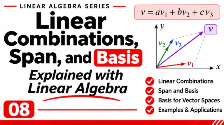
Linear Combinations, Span, and Basis
Learn how vectors can be combined to construct new vectors, understand span geometrically, and explore how bases provide fundamental representations of vector…
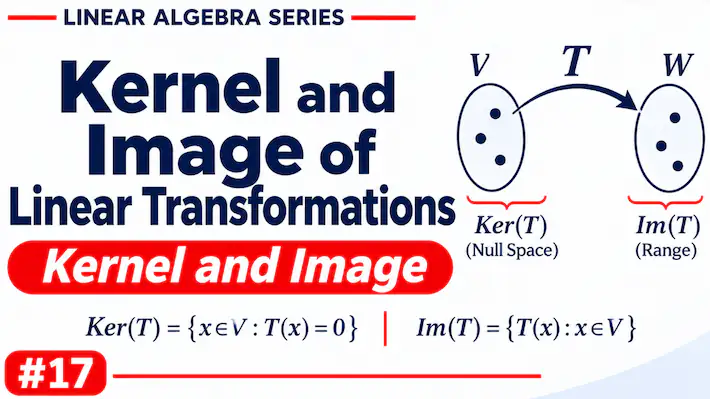
Kernel and Image of Linear Transformations
Understand the kernel and image of linear transformations, how to calculate them using matrices, and how they relate to rank, nullity, injectivity,…

Matrix Factorization: QR Decomposition for Least Squares Problems
Learn QR decomposition, orthogonal matrices, Gram-Schmidt, and how QR factorization solves least squares problems step by step.