
Articles / Linear Algebra · Part 16
Linear Transformations: Mapping Between Vector Spaces and Matrix Representations
Learn what linear transformations are, how they map vectors between vector spaces, and how to represent them using matrices. Explore scaling, rotation, reflection, shear, and step-by-step examples.

1. Introduction
In Linear Algebra, vectors are not just lists of numbers. They can represent positions, directions, data points, forces, or other mathematical quantities.
A linear transformation is a function that maps vectors from one vector space to another while preserving the structure of vector addition and scalar multiplication.
For example, a transformation may:
- Rotate a vector
- Stretch or compress it
- Reflect it
- Shear it
- Map vectors from one space to another
Matrices allow us to represent and calculate these transformations efficiently.
2. What Is a Linear Transformation?
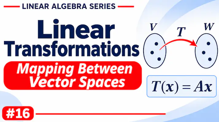
A linear transformation is a function (T) between two vector spaces that preserves vector addition and scalar multiplication.
We write:
\[
T:V\rightarrow W
\]
Where:
- \(V\) is the input vector space.
- \(W\) is the output vector space.
- \(T\) is the transformation.
A transformation is linear if it satisfies two conditions.
Property 1: Additivity
The transformation must preserve vector addition.
\[
\boxed{T(\mathbf{u}+\mathbf{v})=T(\mathbf{u})+T(\mathbf{v})}
\]
This means transforming the sum of two vectors gives the same result as transforming each vector separately and then adding them.
Property 2: Homogeneity
The transformation must preserve scalar multiplication.
\[
\boxed{T(c\mathbf{v})=cT(\mathbf{v})}
\]
Where (c) is any scalar.
This means multiplying a vector by a scalar before transformation gives the same result as multiplying its transformed vector by that scalar.
Both properties must hold for a transformation to be linear.
Together, they can also be expressed as:
\[
\boxed{
T(a\mathbf{u}+b\mathbf{v})
=aT(\mathbf{u})+bT(\mathbf{v})
}
\]
for scalars (a,b).
3. Example of a Linear Transformation
Consider the transformation:
\[
T(x,y)=(2x,3y)
\]
This transformation doubles the (x)-coordinate and triples the (y)-coordinate.
For example:
\[
\begin{bmatrix}
2\
6
\end{bmatrix}
\]
And:
\[
\begin{bmatrix}
6\
3
\end{bmatrix}
\]
The transformation stretches vectors differently along the two coordinate directions.
It is linear because it preserves vector addition and scalar multiplication.
4. Examples of Linear Transformations
A. Scaling
Scaling changes the magnitude of a vector.
For example:
\[
T(x,y)=(2x,2y)
\]
Every vector is multiplied by 2, doubling its magnitude without changing its direction.
The matrix representation is:
\[
A=
\begin{bmatrix}
2&0\\
0&2
\end{bmatrix}
\]
B. Rotation
A rotation transforms vectors by rotating them around the origin.
A rotation by angle \(\theta\) is represented by:
\[
A=
\begin{bmatrix}
\cos\theta&-\sin\theta\\
\sin\theta&\cos\theta
\end{bmatrix}
\]
For a rotation of (90^\circ):
\[
A=
\begin{bmatrix}
0&-1\\
1&0
\end{bmatrix}
\]
Applying it to a vector:
\[
\begin{bmatrix}
0\\
1
\end{bmatrix}
\]
The vector ((1,0)) is rotated to ((0,1)).
C. Reflection
Reflection flips vectors across an axis.
Reflection across the (x)-axis is represented by:
\[
A=
\begin{bmatrix}
1&0\\
0&-1
\end{bmatrix}
\]
Applying it:
\[
\begin{bmatrix}
2\
-3
\end{bmatrix}
\]
The (x)-coordinate remains unchanged, while the (y)-coordinate changes sign.
D. Shearing
A shear transformation shifts one coordinate according to another coordinate.
For example:
\[
A=
\begin{bmatrix}
1&1\\
0&1
\end{bmatrix}
\]
Applying it to:
\[
\begin{bmatrix}
x\
y
\end{bmatrix}
\]
gives:
\[
\begin{bmatrix}
x+y\
y
\end{bmatrix}
\]
The (y)-coordinate remains unchanged, while the (x)-coordinate is shifted by (y).
5. Matrix Representation of Linear Transformations
One of the most useful properties of linear transformations is that they can be represented using matrices.
For a transformation:
\[
T:\mathbb{R}^n\rightarrow\mathbb{R}^m
\]
there exists an (m\times n) matrix (A) such that:
\[
\boxed{T(\mathbf{x})=A\mathbf{x}}
\]
This matrix is called the matrix representation of the transformation with respect to the standard bases.
The matrix allows us to calculate the transformed vector using matrix multiplication.
Example
Consider:
\[
T(x,y)=(2x+y,x-3y)
\]
We can write:
\[
\begin{bmatrix}
2x+y\
x-3y
\end{bmatrix}
\]
Rearranging the expressions:
\[
\boxed{
T(\mathbf{x})=
\begin{bmatrix}
2&1\\
1&-3
\end{bmatrix}
\begin{bmatrix}
x\
y
\end{bmatrix}
}
\]
Therefore, the matrix representation is:
\[
\boxed{
A=
\begin{bmatrix}
2&1\\
1&-3
\end{bmatrix}
}
\]
For the vector:
\[
\mathbf{x}=
\begin{bmatrix}
1\
2
\end{bmatrix}
\]
we obtain:
\[
\begin{aligned}
T(\mathbf{x})
&=
\begin{bmatrix}
2&1\\
1&-3
\end{bmatrix}
\begin{bmatrix}
1\\
2
\end{bmatrix}\\[6pt]
&=
\begin{bmatrix}
2+2\\
1-6
\end{bmatrix}\\[6pt]
&=
\begin{bmatrix}
4\\
-5
\end{bmatrix}
\end{aligned}
\]
Thus, the transformation maps the vector ((1,2)) to ((4,-5)).
6. How to Construct a Transformation Matrix
A transformation matrix can be constructed by determining how the transformation acts on the standard basis vectors.
In \(\mathbb{R}^2\), the standard basis vectors are:
\[
\mathbf{e}_1=
\begin{bmatrix}
1\
0
\end{bmatrix},
\qquad
\mathbf{e}_2=
\begin{bmatrix}
0\
1
\end{bmatrix}
\]
The columns of the matrix are the transformed basis vectors:
\[
\boxed{
A=
\begin{bmatrix}
|&|\
T(\mathbf{e}_1)&T(\mathbf{e}_2)\
|&|
\end{bmatrix}
}
\]
Example
Suppose a transformation is defined as:
\[
T(x,y)=(2x+y,,3x-y)
\]
First, transform the first basis vector:
\[
\begin{bmatrix}
2\
3
\end{bmatrix}
\]
Then transform the second basis vector:
\[
\begin{bmatrix}
1\
-1
\end{bmatrix}
\]
Place these vectors as columns:
\[
\boxed{
A=
\begin{bmatrix}
2&1\\
3&-1
\end{bmatrix}
}
\]
This matrix represents the transformation.
This method is especially useful when a transformation is defined geometrically rather than directly through equations.
7. Transformations Between Different Vector Spaces
A linear transformation does not have to map a vector space to itself.
For example:
\[
T:\mathbb{R}^2\rightarrow\mathbb{R}^3
\]
This means that a two-dimensional input vector is mapped to a three-dimensional output vector.
Consider:
\[
T(x,y)=(x+y,2x,y)
\]
The matrix representation is:
\[
A=
\begin{bmatrix}
1&1\
2&0\
0&1
\end{bmatrix}
\]
This is a (3\times2) matrix because the transformation takes two-dimensional vectors and produces three-dimensional vectors.
For example:
\[
\begin{bmatrix}
3\
2\
2
\end{bmatrix}
\]
This demonstrates how matrices can map vectors between different dimensions.
8. How to Identify a Non-Linear Transformation
Not every transformation is linear.
Consider:
\[
T(x,y)=(x+1,y)
\]
This transformation shifts every vector one unit to the right.
However, it is not linear because:
\[
T(\mathbf{0})\neq\mathbf{0}
\]
For a linear transformation, the zero vector must always map to the zero vector:
\[
\boxed{T(\mathbf{0})=\mathbf{0}}
\]
Here:
\[
T(0,0)=(1,0)
\]
Therefore, the transformation is not linear.
Other examples of non-linear transformations include:
\[
T(x)=x^2
\]
and:
\[
T(x,y)=(xy,x+y)
\]
These transformations do not generally preserve vector addition and scalar multiplication.
9. Applications of Linear Transformations
Linear transformations are used in many areas of mathematics and computer science.
Computer Graphics
Transformations are used to rotate, scale, reflect, and move objects in graphics.
Machine Learning
Linear transformations are fundamental to neural networks, feature transformations, and many mathematical operations used in models.
Robotics
Transformations represent changes in position, orientation, and coordinate systems.
Data Science
Linear transformations help change representations of data, including dimensionality reduction techniques.
Physics
They describe transformations of physical quantities, coordinate systems, and mathematical models.
10. Summary
A linear transformation maps vectors from one vector space to another while preserving vector addition and scalar multiplication.
The two defining properties are:
\[
T(\mathbf{u}+\mathbf{v})=T(\mathbf{u})+T(\mathbf{v})
\]
\[
T(c\mathbf{v})=cT(\mathbf{v})
\]
Every linear transformation between finite-dimensional vector spaces can be represented by a matrix when bases are chosen.
\[
T(\mathbf{x})=A\mathbf{x}
\]
The columns of the transformation matrix can be obtained by transforming the standard basis vectors.
Linear transformations form the foundation of many important applications, including computer graphics, robotics, Machine Learning, and data analysis.
They also prepare us for the next topic: understanding the kernel and image of linear transformations.
Quick quiz
5 questionsOriginally published at farhanpaal.com — https://farhanpaal.com/articles/linear-transformations-mapping-between-vector-spaces-and-matrix-representations/
Keep a copy
Read offline as a printout or PDF.
farhanpaal.comKeep reading

Role of Eigenvalues in Markov Models and Google’s PageRank Algorithm
Learn how Markov models work, explore steady-state probabilities, and discover how eigenvalues and eigenvectors power Google's PageRank algorithm.
Determinants and Matrix Inverse Explained: From Cofactors to Invertibility
Learn determinants, minors, cofactors, invertibility, and matrix inverses with clear examples, row reduction, and practical applications in linear algebra.
Application: Solving Linear Systems Using Matrix Inverses
Learn how to solve systems of linear equations using matrix inverses, with step-by-step examples, determinant calculations, and practical Python applications.