
Graphs: Terminology, Representations, and Traversal Techniques (BFS & DFS)
Learn what graphs are, how they are represented using adjacency matrices and lists, and how BFS and DFS traverse graphs.

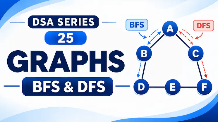
1. Introduction to Graphs
In previous articles, we studied trees, which represent hierarchical relationships. However, many real-world relationships are not hierarchical.
For example:
- Cities connected by roads
- People connected through friendships
- Computers connected in a network
- Websites connected through hyperlinks
These relationships can be represented using a Graph.
A graph is a non-linear data structure consisting of a set of vertices and edges connecting them.
Mathematically, a graph is represented as:
\[
G = (V,E)
\]
Where:
- (V) represents the set of vertices (nodes).
- (E) represents the set of edges (connections between vertices).
For example, if five cities are connected by roads, the cities represent vertices and the roads represent edges.
Unlike trees, graphs do not necessarily have a root, and they may contain cycles or multiple paths between vertices.
2. Basic Graph Terminologies
Vertex and Edge
A Vertex is an individual element of a graph.
An Edge is a connection between two vertices.
For example, if A and B are connected, the edge can be represented as (A-B) in an undirected graph.
Adjacent Vertices
Two vertices are adjacent if they are directly connected by an edge.
If A is connected to B, then A and B are adjacent.
Degree
The degree of a vertex is the number of edges connected to it in an undirected graph.
For example, if A is connected to B, C, and D, then:
\[
\deg(A)=3
\]
In a directed graph, degree is divided into:
- In-degree: Number of incoming edges.
- Out-degree: Number of outgoing edges.
Path
A path is a sequence of vertices connected through edges.
For example:
A → B → D → E
represents a path from A to E.
Cycle
A cycle is a path that starts and ends at the same vertex.
For example:
A → B → C → A
Connected Graph
An undirected graph is connected if a path exists between every pair of vertices.
If some vertices cannot be reached from others, the graph is disconnected.
Connected Component
A connected component is a group of vertices in an undirected graph where every vertex is reachable from the others within that group.
Directed and Undirected Graphs
Undirected Graph: Edges have no direction. If A is connected to B, movement is possible in both directions.
Directed Graph (Digraph): Edges have a direction. A connection from A to B does not necessarily mean B can connect back to A.
Weighted Graph
A weighted graph assigns a value to each edge, such as distance, cost, time, or network strength.
For example, a road between two cities may have a distance of 25 km.
3. Graph Representation
A graph must be stored in memory before algorithms can operate on it. Two commonly used representations are the Adjacency Matrix and Adjacency List.
Consider the following graph:
Vertices: A, B, C, D, E
Edges: A-B, A-C, B-D, C-D, C-E
Adjacency Matrix
An adjacency matrix is a two-dimensional array used to represent connections between vertices.
If an edge exists between two vertices, we store 1; otherwise, we store 0.
For our example:
| A | B | C | D | E | |
|---|---|---|---|---|---|
| A | 0 | 1 | 1 | 0 | 0 |
| B | 1 | 0 | 0 | 1 | 0 |
| C | 1 | 0 | 0 | 1 | 1 |
| D | 0 | 1 | 1 | 0 | 0 |
| E | 0 | 0 | 1 | 0 | 0 |
Since the graph is undirected, the matrix is symmetric.
Advantages:
- Checking whether an edge exists takes (O(1)) time.
- Simple to implement.
- Useful for dense graphs.
Disadvantages:
- Requires \(O(V^2)\) memory, even when very few edges exist.
- Finding all neighbors of a vertex requires checking an entire row.
Adjacency List
An adjacency list stores each vertex along with a list of its neighboring vertices.
For the same graph:
| Vertex | Neighbors |
|---|---|
| A | B, C |
| B | A, D |
| C | A, D, E |
| D | B, C |
| E | C |
For an undirected graph, each edge appears in the neighbor lists of both connected vertices.
Advantages:
- Requires \(O(V+E)\) space.
- Efficient for exploring neighboring vertices.
- Suitable for sparse graphs.
Disadvantages:
- Checking whether a particular edge exists may require searching through a vertex’s neighbor list.
Comparison
| Feature | Adjacency Matrix | Adjacency List |
|---|---|---|
| Memory | \(O(V^2)\) | \(O(V+E)\) |
| Edge checking | \(O(1)\) | \(O(\deg(V))\) in a typical list |
| Finding neighbors | \(O(V)\) | \(O(\deg(V))\) |
| Best suited for | Dense graphs | Sparse graphs |
4. Graph Traversal
Graph traversal is the process of systematically visiting vertices of a graph.
Since graphs may contain cycles and multiple paths to the same vertex, we maintain a visited array or set to avoid visiting the same vertex repeatedly.
The two fundamental traversal techniques are:
- Breadth-First Search (BFS)
- Depth-First Search (DFS)
We will use the same graph throughout this section.
Vertices: A, B, C, D, E, F
Edges: A-B, A-C, B-D, C-D, C-E, E-F
5. Breadth-First Search (BFS)
Breadth-First Search explores a graph level by level.
It first visits the starting vertex, then all its immediate neighbors, followed by the neighbors of those vertices.
BFS uses a Queue, which follows FIFO (First In, First Out).
Working of BFS
Suppose we start from vertex A.
- Mark A as visited and insert it into the queue.
- Remove A from the queue and visit it.
- Add its unvisited neighbors B and C.
- Remove B and add its unvisited neighbor D.
- Remove C and add its unvisited neighbor E.
- Remove D. No new vertex is added.
- Remove E and add F.
- Remove F. The queue becomes empty, so traversal ends.
The traversal order is:
A → B → C → D → E → F
BFS Algorithm
BFS(graph, start):

    create a queue
    mark start as visited
    enqueue start

    while queue is not empty:

        vertex = dequeue
        visit vertex

        for each neighbor of vertex:

            if neighbor is not visited:

                mark neighbor as visited
                enqueue neighbor
Why BFS Uses a Queue
A queue ensures that vertices discovered earlier are processed first.
Therefore, BFS explores vertices at distance 1 from the starting vertex before vertices at distance 2, and so on.
This makes BFS useful for finding the shortest path in an unweighted graph, where each edge is considered to have equal cost.
Time Complexity
Using an adjacency list:
\[
O(V+E)
\]
Each vertex is visited once, and the edges are examined during traversal.
6. Depth-First Search (DFS)
Depth-First Search explores as deeply as possible along one path before returning to explore another path.
It uses a Stack, or recursion which internally uses the call stack.
Working of DFS
Starting from A:
- Visit A.
- Move to B.
- From B, move to D.
- From D, move to C.
- From C, move to E.
- From E, move to F.
- F has no unvisited neighbors, so backtrack.
- Continue backtracking until all reachable vertices have been visited.
One possible traversal order is:
A → B → D → C → E → F
The exact traversal order may change depending on the order in which neighbors are selected.
DFS Algorithm
DFS(graph, vertex):

    mark vertex as visited
    visit vertex

    for each neighbor of vertex:

        if neighbor is not visited:

            DFS(graph, neighbor)
Why DFS Uses a Stack
DFS keeps moving deeper into the graph. When it reaches a vertex with no unvisited neighbors, it returns to the previous vertex and continues exploring.
This behavior follows the LIFO (Last In, First Out) principle of a stack.
Time Complexity
Using an adjacency list:
\[
O(V+E)
\]
Each vertex is visited once, and edges are examined during the traversal.
7. BFS vs DFS
| Feature | BFS | DFS |
|---|---|---|
| Full form | Breadth-First Search | Depth-First Search |
| Exploration | Level by level | As deep as possible |
| Data structure | Queue | Stack / Recursion |
| Shortest path | Finds shortest path in an unweighted graph | Does not guarantee shortest path |
| Memory | May store many vertices of a level | Stores the current path and pending branches |
| Applications | Shortest paths, level exploration | Cycle detection, path exploration, connected components |
Both algorithms have a time complexity of (O(V+E)) when implemented using adjacency lists.
8. Applications of Graphs
Graphs are widely used in computer science and real-world systems.
- Social Networks: Representing relationships between people.
- Maps and Navigation: Representing cities, roads, and routes.
- Computer Networks: Representing computers, routers, and connections.
- Web Search: Representing links between web pages.
- Dependency Management: Representing prerequisites between tasks or courses.
- Recommendation Systems: Representing connections between users and products.
BFS and DFS are foundational algorithms used in many graph-related problems.
Graphs are powerful data structures used to represent connections and relationships between objects.
In this article, we learned the basic graph terminology, how graphs are represented using adjacency matrices and adjacency lists, and how BFS and DFS traverse graphs.
BFS explores level by level using a queue, while DFS explores deeper using a stack or recursion.
In the next article, we will study Minimum Spanning Trees and Shortest Path Algorithms, which use graphs to solve optimization problems such as finding efficient network connections and shortest routes.
Quick quiz
5 questionsOriginally published at farhanpaal.com — https://farhanpaal.com/articles/graphs-terminology-representations-and-traversal-techniques-bfs-dfs/
Keep a copy
Read offline as a printout or PDF.
farhanpaal.comKeep reading
Applications of Stacks: Parenthesis Checker, Infix to Postfix, and Evaluation
Explore three important applications of stacks: balanced parenthesis checking, Infix to Postfix conversion, and Postfix expression evaluation, with step-by-step examples and C…

Space and Time Complexity in DSA
Understand time complexity, space complexity, Big O notation, and how to analyse algorithm efficiency with simple examples.

Arrays: Understanding the Basics
Learn the basics of arrays, including indexing, memory representation, accessing, updating, traversing, insertion, and deletion with simple C examples.