
Articles / Linear Algebra · Part 19
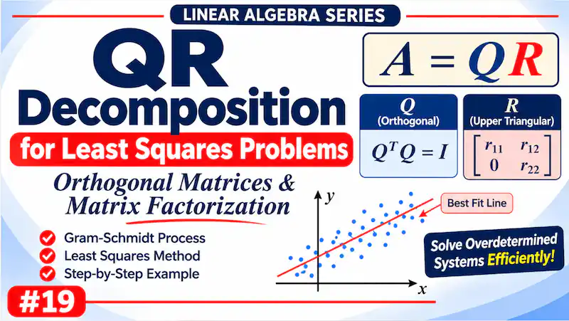
Matrix Factorization: QR Decomposition for Least Squares Problems
Learn QR decomposition, orthogonal matrices, Gram-Schmidt, and how QR factorization solves least squares problems step by step.

1. Introduction
In many real-world problems, we deal with systems of equations that do not have an exact solution.
For example, when collecting data from experiments, measurements may contain errors. A system may have more equations than unknowns, making it impossible to satisfy every equation exactly.
In such cases, we often look for the solution that minimizes the overall error.
QR Decomposition is a matrix factorization technique that helps us solve these problems efficiently and reliably.
It expresses a matrix as the product of two matrices:
- Q: An orthogonal matrix (or a matrix with orthonormal columns).
- R: An upper triangular matrix.
\[
\boxed{A=QR}
\]
QR decomposition is particularly useful in least squares problems, data fitting, numerical computation, and machine learning.
2. What Is QR Decomposition?
QR decomposition represents a matrix (A) as:
\[
A=QR
\]
where:
Matrix Q
The columns of (Q) are orthonormal vectors.
This means:
- Each column has a length of 1.
- Different columns are perpendicular to each other.
Mathematically:
\[
Q^TQ=I
\]
Matrix R
\(R\) is an upper triangular matrix, meaning all entries below its main diagonal are zero.
For example:
\[
R=
\begin{bmatrix}
r_{11}&r_{12}&r_{13}\\
0&r_{22}&r_{23}\\
0&0&r_{33}
\end{bmatrix}
\]
The advantage of this factorization is that orthogonal matrices have useful mathematical properties that make calculations more stable and easier to perform.
3. Understanding QR Decomposition with an Example
Consider the matrix:
\[
A=
\begin{bmatrix}
1&1\\
1&0\\
0&1
\end{bmatrix}
\]
We want to decompose it into:
\[
A=QR
\]
We can use the Gram-Schmidt process to convert the columns of (A) into orthonormal vectors.
The columns of (A) are:
\[
\mathbf{a}_1=
\begin{bmatrix}
1\\1\\0
\end{bmatrix},
\qquad
\mathbf{a}_2=
\begin{bmatrix}
1\\0\\1
\end{bmatrix}
\]
Step 1: Find the first orthonormal vector
First, calculate the length of \(\mathbf{a}_1\):
\[
\mathbf{a}_1=\sqrt{1^2+1^2+0^2}=\sqrt2
\]
Normalize the vector:
\[
\frac{1}{\sqrt2}
\begin{bmatrix}
1\\1\\0
\end{bmatrix}
\]
Step 2: Remove the projection from the second vector
We need to remove the component of \(\mathbf{a}_2\) that lies in the direction of \(\mathbf{q}_1\).
The projection coefficient is:
\[
r_{12}=\mathbf{q}_1^T\mathbf{a}_2
\]
\[
r_{12}=\frac{1}{\sqrt2}(1+0+0)
=\frac{1}{\sqrt2}
\]
Now subtract the projection:
\[
\mathbf{u}_2=
\mathbf{a}_2-r_{12}\mathbf{q}_1
\]
\[
\mathbf{u}_2=
\begin{bmatrix}
1\\0\\1
\end{bmatrix}
–
\frac12
\begin{bmatrix}
1\\1\\0
\end{bmatrix}
\]
\[
\mathbf{u}_2=
\begin{bmatrix}
1/2\\-1/2\\1
\end{bmatrix}
\]
Step 3: Normalize the second vector
Calculate its length:
\[
\|\mathbf{u}_2\|=
\sqrt{\frac14+\frac14+1}
=\frac{\sqrt6}{2}
\]
Therefore:
\[
\mathbf{q}_2=
\frac{\mathbf{u}_2}{\|\mathbf{u}_2\|}
=
\frac{1}{\sqrt6}
\begin{bmatrix}
1\\-1\\2
\end{bmatrix}
\]
Now our two orthonormal vectors are:
\[
\mathbf{q}_1=
\frac{1}{\sqrt2}
\begin{bmatrix}
1\\1\\0
\end{bmatrix},
\qquad
\mathbf{q}_2=
\frac{1}{\sqrt6}
\begin{bmatrix}
1\\-1\\2
\end{bmatrix}
\]
4. Constructing Q and R
The columns of (Q) are the orthonormal vectors we calculated.
\[
Q=
\begin{bmatrix}
\frac1{\sqrt2}&\\frac1{\sqrt6}\
\frac1{\sqrt2}&-\\frac1{\sqrt6}\
0&\frac2{\sqrt6}
\end{bmatrix}
\]
The entries of (R) are calculated using the projections and vector lengths:
\[
r_{11}=|\mathbf{a}_1|=\sqrt2
\]
\[
r_{12}=\mathbf{q}_1^T\mathbf{a}_2
=\frac1{\sqrt2}
\]
\[
r_{22}=|\mathbf{u}_2|=\frac{\sqrt6}{2}
\]
Therefore:
\[
R=
\begin{bmatrix}
\sqrt2&\\frac1{\sqrt2}\
0&\\frac{\sqrt6}{2}
\end{bmatrix}
\]
Our final decomposition is:
\[
\boxed{A=QR}
\]
where:
\[
Q=
\begin{bmatrix}
\frac1{\sqrt2}&\\frac1{\sqrt6}\
\frac1{\sqrt2}&-\\frac1{\sqrt6}\
0&\frac2{\sqrt6}
\end{bmatrix}
\]
and:
\[
R=
\begin{bmatrix}
\sqrt2&\\frac1{\sqrt2}\
0&\\frac{\sqrt6}{2}
\end{bmatrix}
\]
5. What Is a Least Squares Problem?
Suppose we have a system:
\[
A\mathbf{x}=\mathbf{b}
\]
If the system has no exact solution, we look for an approximate solution (\hat{\mathbf{x}}) that minimizes the error.
The error or residual vector is:
\[
\mathbf{e}=\mathbf{b}-A\hat{\mathbf{x}}
\]
The least squares method finds the value of (\hat{\mathbf{x}}) that minimizes the squared length of this residual:
\[
\boxed{
\min_{\mathbf{x}}|\mathbf{b}-A\mathbf{x}|^2
}
\]
This means we try to find the solution whose predicted values are as close as possible to the actual observations.
6. Solving Least Squares Using QR Decomposition
Consider the system:
\[
A\mathbf{x}\approx\mathbf{b}
\]
where:
\[
A=
\begin{bmatrix}
1&1\\
1&0\\
0&1
\end{bmatrix},
\qquad
\mathbf{b}=
\begin{bmatrix}
1\\2\\3
\end{bmatrix}
\]
We already have:
\[
A=QR
\]
Therefore:
\[
QR\mathbf{x}\approx\mathbf{b}
\]
Since the columns of (Q) are orthonormal, we can multiply by \(Q^T\):
\[
Q^TQ R\mathbf{x}=Q^T\mathbf{b}
\]
Because:
\[
Q^TQ=I
\]
we get:
\[
\boxed{R\mathbf{x}=Q^T\mathbf{b}}
\]
This is the key step in solving least squares problems using QR decomposition.
Step 1: Calculate \(Q^T\mathbf{b}\)
Using our (Q) matrix:
\[
\begin{bmatrix}
\frac1{\sqrt2}&\\frac1{\sqrt2}&0\\
\frac1{\sqrt6}&-\\frac1{\sqrt6}&\\frac2{\sqrt6}
\end{bmatrix}
\begin{bmatrix}
1\\2\\3
\end{bmatrix}
\]
\[
\begin{bmatrix}
\frac3{\sqrt2}\\
\frac5{\sqrt6}
\end{bmatrix}
\]
Step 2: Solve \(R\mathbf{x}=Q^T\mathbf{b}\)
\[
\begin{bmatrix}
\frac3{\sqrt2}\\
\frac5{\sqrt6}
\end{bmatrix}
\]
From the second equation:
\[
\frac{\sqrt6}{2}x_2=\frac5{\sqrt6}
\]
\[
x_2=\frac53
\]
Substitute into the first equation:
\[
\sqrt2x_1+\frac1{\sqrt2}\left(\frac53\right)
=\frac3{\sqrt2}
\]
Multiplying by \(\sqrt2\):
\[
2x_1+\frac53=3
\]
\[
2x_1=\frac43
\]
\[
x_1=\frac23
\]
Therefore, the least squares solution is:
\[
\boxed{
\hat{\mathbf{x}}=
\begin{bmatrix}
\frac23\
\frac53
\end{bmatrix}
}
\]
7. Applications of QR Decomposition
QR decomposition is useful in many fields.
Data Fitting
When fitting a line or curve to experimental data, QR decomposition can help calculate the parameters that minimize the fitting error.
Machine Learning
It can be used in numerical optimization, regression, and solving systems that arise during model training.
Scientific Computing
QR decomposition is used in numerical algorithms where accuracy and stability are important.
Engineering
Engineers use least squares methods to estimate parameters from measurements, sensor data, and experimental observations.
Numerical Mathematics
QR algorithms are also used in computing eigenvalues and solving various numerical problems.
QR decomposition expresses a matrix as the product of an orthogonal matrix (Q) and an upper triangular matrix (R).
\[
A=QR
\]
Its major advantage is that it makes least squares problems easier to solve while often providing better numerical stability than directly solving the normal equations.
By transforming the problem into:
\[
R\mathbf{x}=Q^T\mathbf{b}
\]
we can efficiently find the solution that minimizes the error.
Key takeaway: QR decomposition is particularly useful when a system of equations has no exact solution and we need the best approximate solution.
Quick quiz
5 questionsOriginally published at farhanpaal.com — https://farhanpaal.com/articles/matrix-factorization-qr-decomposition-for-least-squares-problems/
Keep a copy
Read offline as a printout or PDF.
farhanpaal.comKeep reading

Singular Value Decomposition (SVD)
Learn Singular Value Decomposition (SVD), calculate singular values and vectors, and explore its applications in compression, machine learning, and dimensionality reduction.

Real-World Applications of Linear Independence in Error Detection and Coding Theory
Understand how linear independence powers error detection and coding theory. Explore parity bits, linear codes, parity-check matrices, syndromes, and applications in communication…

Linear Transformations: Mapping Between Vector Spaces and Matrix Representations
Learn what linear transformations are, how they map vectors between vector spaces, and how to represent them using matrices. Explore scaling, rotation,…