
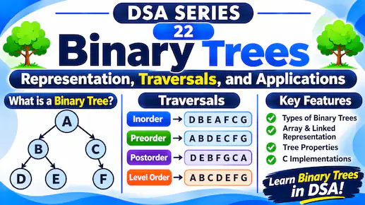
Binary Trees: Representation, Traversals, and Applications
Learn binary tree types, array and linked representations, and inorder, preorder, postorder, and level order traversals with diagrams and C examples.

In the previous article, we learned the basic terminology and properties of trees.
Now let’s explore a special type of tree called a Binary Tree.
Binary trees are widely used in computer science for organising data, searching, sorting, and representing expressions.
1. What Is a Binary Tree?
A Binary Tree is a tree data structure in which each node can have at most two children.
These children are called:
- Left Child
- Right Child
A node can have no children, one child, or two children.
Example:
          A
         / \
        B   C
       / \   \
      D   E   F
Here:
- A is the root node.
- B is the left child of A.
- C is the right child of A.
- B has two children: D and E.
- C has only one child: F.
Notice that no node has more than two children.
This is what makes it a Binary Tree.
2. Types of Binary Trees
Binary trees can be classified into different types based on how their nodes are arranged.
A. Full Binary Tree
A Full Binary Tree is a binary tree in which every node has either zero or exactly two children.
        A
       / \
      B   C
     / \
    D   E
Here, every node has either two children or no children.
B. Complete Binary Tree
A Complete Binary Tree is a binary tree in which:
- Every level is completely filled except possibly the last level.
- The last level is filled from left to right without gaps.
        A
       / \
      B   C
     / \  /
    D  E F
C. Perfect Binary Tree
A Perfect Binary Tree is a binary tree in which:
- Every internal node has exactly two children.
- All leaf nodes are at the same level.
        A
       / \
      B   C
     / \ / \
    D  E F  G
D. Skewed Binary Tree
A Skewed Binary Tree is a tree in which each node has only one child, forming a chain-like structure.
Left-skewed:
        A
       /
      B
     /
    C
   /
  D
Right-skewed:
    A
     \
      B
       \
        C
         \
          D
These trees resemble linked lists because each node has only one child.
3. Representation of Binary Trees
A binary tree can be stored in memory mainly in two ways:
- Array Representation
- Linked Representation
Let’s understand both.
A. Array Representation
In this method, we store the tree elements inside an array.
Consider this binary tree:
          A
         / \
        B   C
       / \   \
      D   E   F
We store its elements level by level:
Index:    0   1   2   3   4   5   6
Array:   [A,  B,  C,  D,  E,  -,  F]
Here, - represents an empty position.
Using a zero-based array index, we can find the positions of a node’s children:
For a node at index i:
- Left child =
2i + 1 - Right child =
2i + 2 - Parent =
(i - 1) / 2using integer division, for non-root nodes.
Example:
For node B, which is at index 1:
- Left child index =
2(1) + 1 = 3→ D - Right child index =
2(1) + 2 = 4→ E
Advantages:
- Easy to access parent and child positions using index calculations.
- Efficient for complete binary trees.
Disadvantage:
For trees with many missing positions, an array may waste memory storing empty positions.
B. Linked Representation
In this method, each node contains three parts:
- Data
- Pointer to the left child
- Pointer to the right child
A pointer stores the address of another node.
Node Structure in C:
struct Node {
    int data;
    struct Node *left;
    struct Node *right;
};
Here:
datastores the node’s value.leftstores the address of its left child.rightstores the address of its right child.
If a node has no left or right child, the corresponding pointer stores NULL.
This representation is flexible because nodes can be created and connected as needed.
Advantages:
- Memory is allocated as nodes are created.
- No need to reserve empty array positions.
- Convenient for trees that change their shape.
Disadvantage:
- Each node requires extra memory for two pointers.
- Accessing a particular node may require moving through the tree.
4. Tree Traversal
Now that we understand how binary trees are organised and stored, let’s learn how to visit their nodes.
Tree Traversal is the process of visiting every node of a tree in a particular order.
Consider this binary tree:
          A
         / \
        B   C
       / \ / \
      D  E F  G
There are three common depth-first traversal methods:
- Inorder
- Preorder
- Postorder
The difference between them is the order in which we visit the root, left subtree, and right subtree.
A. Inorder Traversal (Left → Root → Right)
In Inorder Traversal, we:
- Visit the left subtree.
- Visit the root.
- Visit the right subtree.
For our example:
          A
         / \
        B   C
       / \ / \
      D  E F  G
The visiting order is:
- First, visit the left subtree of A: D, B, E.
- Then, visit A.
- Finally, visit the right subtree of A: F, C, G.
Result:
D → B → E → A → F → C → GB. Preorder Traversal (Root → Left → Right)
In Preorder Traversal, we:
- Visit the root.
- Visit the left subtree.
- Visit the right subtree.
For our example:
- First, visit A.
- Then, visit the left subtree: B, D, E.
- Finally, visit the right subtree: C, F, G.
Result:
A → B → D → E → C → F → GC. Postorder Traversal (Left → Right → Root)
In Postorder Traversal, we:
- Visit the left subtree.
- Visit the right subtree.
- Visit the root.
For our example:
- First, visit the left subtree: D, E, B.
- Then, visit the right subtree: F, G, C.
- Finally, visit A.
Result:
D → E → B → F → G → C → AQuick Comparison
| Traversal | Visiting Order | Result |
|---|---|---|
| Inorder | Left → Root → Right | D B E A F C G |
| Preorder | Root → Left → Right | A B D E C F G |
| Postorder | Left → Right → Root | D E B F G C A |
A simple way to remember:
- Inorder: Root comes in between.
- Preorder: Root comes first.
- Postorder: Root comes last.
5. Implementing Tree Traversals in C
Let’s implement the three traversal methods using the linked representation.
First, we define a node:
struct Node {
    char data;
    struct Node *left;
    struct Node *right;
};
Inorder Function
void inorder(struct Node *root) {
    if (root == NULL)
        return;

    inorder(root->left);
    printf("%c ", root->data);
    inorder(root->right);
}
Preorder Function
void preorder(struct Node *root) {
    if (root == NULL)
        return;

    printf("%c ", root->data);
    preorder(root->left);
    preorder(root->right);
}
Postorder Function
void postorder(struct Node *root) {
    if (root == NULL)
        return;

    postorder(root->left);
    postorder(root->right);
    printf("%c ", root->data);
}
Notice that all three functions follow the same structure.
The only difference is where the printf() statement appears.
- Inorder: Between the two recursive calls.
- Preorder: Before the recursive calls.
- Postorder: After the recursive calls.
The condition root == NULL stops the function when there is no node to visit.
These functions use recursion, which we studied in the previous article.
6. Level Order Traversal
Apart from the three depth-first methods, there is another important traversal called Level Order Traversal.
In this method, we visit nodes level by level, starting from the root.
Consider the same tree:
          A
         / \
        B   C
       / \ / \
      D  E F  G
We visit:
- Level 1: A
- Level 2: B, C
- Level 3: D, E, F, G
Result:
A → B → C → D → E → F → GLevel Order Traversal uses a Queue to keep track of which node should be visited next.
We will explore queues in detail in our earlier queue articles, and their use in tree traversal will become clearer as we study more advanced tree operations.
7. Applications of Binary Trees
Binary trees are used in several important areas of computer science.
- Binary Search Trees: Organising data to support searching, insertion, and deletion.
- Expression Trees: Representing mathematical expressions such as
(A + B) * C. - Heaps: Supporting priority queues and heap sort.
- Huffman Coding: Building trees used in data compression.
- Decision Trees: Representing decisions and their possible outcomes.
We will explore some of these structures in upcoming articles.
A Binary Tree is a non-linear data structure in which each node can have at most two children.
We learned its main types, two ways of representing it in memory, and four important traversal methods.
The three depth-first traversals differ only in when the root is visited:
- Inorder: Left → Root → Right
- Preorder: Root → Left → Right
- Postorder: Left → Right → Root
Level Order Traversal visits nodes one level at a time.
In the next article, we’ll explore Threaded Binary Trees, AVL Trees, and M-Way Search Trees, where we’ll learn how different tree structures improve memory usage and searching efficiency.
Further reading:· GeeksforGeeks – Tree Traversals
Originally published at farhanpaal.com — https://farhanpaal.com/articles/binary-trees-representation-traversals-and-applications/
Keep a copy
Read offline as a printout or PDF.
farhanpaal.comKeep reading
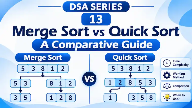
Merge Sort and Quick Sort: A Comparative Guide
Understand how Merge Sort and Quick Sort work with step-by-step examples, C implementations, and a comparison of their time and space complexity.
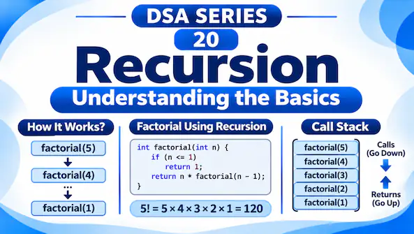
Recursion: Understanding the Basics
Understand recursion, base cases, recursive calls, and the call stack. Learn how to trace recursive functions and calculate factorial using simple C…
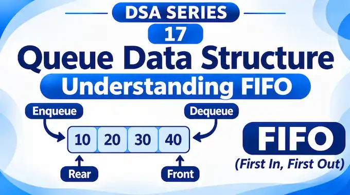
Queue Data Structure: Understanding FIFO
Understand the Queue data structure and its FIFO principle. Learn Enqueue, Dequeue, Front, and Rear operations with simple examples, C implementation, and…