
Articles / Linear Algebra · Part 14
Introduction to Principal Component Analysis (PCA) and Dimensionality Reduction
Understand Principal Component Analysis (PCA), dimensionality reduction, eigenvectors, and eigenvalues. Learn how PCA identifies important directions in data, reduces features, and preserves variance through practical examples.

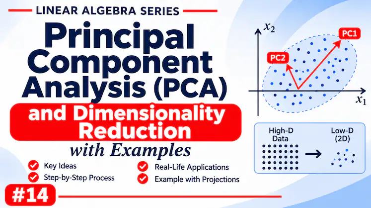
In Machine Learning and Data Science, datasets can contain hundreds or even thousands of features.
For example, a dataset used to analyze students might contain:
- Study hours
- Attendance
- Test scores
- Assignment scores
- Sleep duration
- Time spent on social media
Having more features does not always mean having more useful information. Some features may be strongly related to each other, while others may contribute very little to the overall pattern.
This creates a problem: working with too many dimensions can make data harder to visualize, analyze, and process.
Principal Component Analysis (PCA) is a technique used to reduce the number of dimensions in a dataset while retaining as much important information as possible.
It helps us represent complex data in a simpler form.
2. What Is Dimensionality Reduction?
Dimensionality refers to the number of features or variables used to represent each data point.
For example:
| Data Point | Height | Weight | Age |
|---|---|---|---|
| Person 1 | 170 cm | 65 kg | 20 |
| Person 2 | 180 cm | 80 kg | 22 |
| Person 3 | 160 cm | 55 kg | 19 |
Each person is represented using three features. Therefore, this dataset has three dimensions.
Dimensionality reduction is the process of reducing the number of features while trying to preserve the most useful information.
For example, instead of representing each person using height, weight, and age, we might transform the data into two new features that capture most of the variation in the dataset.
This can make the data easier to visualize and process.
3. Why Do We Need Dimensionality Reduction?
Dimensionality reduction is useful for several reasons.
A. Simplifying Data
Datasets with many features can be difficult to understand. Reducing the number of dimensions makes the data simpler to analyze.
B. Visualization
Humans can easily visualize two-dimensional and three-dimensional data.
However, visualizing data with 50 or 100 features is difficult.
Dimensionality reduction can help transform high-dimensional data into two or three dimensions so that patterns can be visualized.
C. Removing Redundant Information
Some features may contain similar information.
For example, height measured in centimeters and height measured in meters represent the same underlying information.
Similarly, in real datasets, multiple features may be strongly correlated.
Dimensionality reduction can help combine related information into fewer features.
D. Computational Efficiency
Reducing the number of features can decrease the computational cost of certain Machine Learning algorithms.
It may also help reduce noise and improve the performance of some models, although this is not guaranteed.
4. What Is Principal Component Analysis?
Principal Component Analysis (PCA) is a mathematical technique that transforms a dataset into a new set of features called principal components.
These components are arranged according to how much variance they capture from the original data.
The first principal component captures the largest possible amount of variance.
The second principal component captures the largest remaining amount of variance while being perpendicular to the first.
The third captures the largest remaining variance while being perpendicular to the first two, and so on.
In this way, PCA identifies the directions in which the data varies the most.
Instead of using the original features, we can represent the data using a smaller number of principal components.
5. Understanding PCA Intuitively
Imagine a dataset containing the heights and weights of many people.
Generally, taller people tend to weigh more, so height and weight may be correlated.
If we plot these data points, they may form a pattern extending diagonally across the graph.
This means that much of the information in the two original features may be represented by a single direction.
PCA identifies this direction.
The first principal component points in the direction of maximum variance in the data.
If most of the data’s variation is along this direction, we may represent the dataset using only this component, reducing the dimensions from two to one while preserving much of the variation.
This is the basic idea behind PCA.
6. The Role of Eigenvectors and Eigenvalues
PCA relies on concepts we studied in previous articles: eigenvectors and eigenvalues.
After preparing the data, PCA calculates a covariance matrix that describes how the features vary and how they are related to each other.
The eigenvectors of this covariance matrix represent the principal directions of the data.
The corresponding eigenvalues indicate how much variance is associated with each direction.
- A large eigenvalue means that the corresponding principal component captures a large amount of variance.
- A small eigenvalue means that the component captures relatively little variance.
Therefore, PCA sorts the principal components according to their eigenvalues.
The components with the largest eigenvalues are generally the most important for representing the data.
This connects PCA directly to our previous articles on eigenvalues, eigenvectors, and diagonalization.
7. How PCA Works: Step-by-Step
PCA generally follows these steps.
Step 1: Prepare the Dataset
Arrange the dataset into a matrix where rows represent observations and columns represent features.
For example:
\[
X=
\begin{bmatrix}
x_{11}&x_{12}&x_{13}\\
x_{21}&x_{22}&x_{23}\\
x_{31}&x_{32}&x_{33}\\
\vdots&\vdots&\vdots&\vdots
\end{bmatrix}
\]
Each row represents a data point, and each column represents a feature.
Step 2: Center the Data
Calculate the mean of each feature and subtract it from the corresponding values.
This makes the mean of each feature approximately zero.
The centered data is important because PCA analyzes variation around the mean.
If the features have significantly different scales, standardization may also be appropriate before PCA.
For example, height measured in centimeters and income measured in thousands can have very different numerical scales.
Step 3: Calculate the Covariance Matrix
The covariance matrix describes how features vary together.
For a centered dataset (X) with (n) observations, the sample covariance matrix is:
\[
C=\frac{1}{n-1}X^TX
\]
The diagonal entries represent the variances of individual features.
The off-diagonal entries represent the covariances between pairs of features.
A positive covariance indicates that two features tend to increase together, while a negative covariance indicates that they tend to move in opposite directions.
Step 4: Find Eigenvalues and Eigenvectors
Calculate the eigenvalues and eigenvectors of the covariance matrix:
\[
C\mathbf{v}=\lambda\mathbf{v}
\]
The eigenvectors represent the principal directions.
The eigenvalues indicate how much variance each principal direction captures.
Step 5: Sort the Principal Components
Arrange the eigenvalues from largest to smallest.
The corresponding eigenvectors are arranged in the same order.
The first principal component corresponds to the largest eigenvalue, the second to the next largest, and so on.
Step 6: Select the Components
Choose the number of principal components you want to retain.
For example, if a dataset contains 10 features, you might choose to retain only the first two or three principal components if they preserve a sufficiently large proportion of the variance.
Step 7: Transform the Data
Create a matrix (W) containing the selected eigenvectors.
Transform the centered data:
\[
Z=XW
\]
Here:
- (X) is the centered original dataset.
- (W) contains the selected principal component directions.
- (Z) is the transformed dataset.
The transformed dataset has fewer dimensions than the original dataset when fewer components are selected.
8. Explained Variance
Explained variance tells us how much of the dataset’s total variance is captured by a principal component.
For a principal component with eigenvalue \(\lambda_i\):
\[
\text{Explained Variance Ratio}_i=
\frac{\lambda_i}{\sum_{j=1}^{n}\lambda_j}
\]
The result tells us what proportion of the total variance is captured by that component.
Example
Suppose a dataset has four principal components with eigenvalues:
\[
\lambda_1=6,\quad
\lambda_2=3,\quad
\lambda_3=0.8,\quad
\lambda_4=0.2
\]
The total variance is:
\[
6+3+0.8+0.2=10
\]
The first principal component captures:
\[
\frac{6}{10}\times100=60%
\]
The second principal component captures:
\[
\frac{3}{10}\times100=30%
\]
Together, the first two components capture:
\[
60%+30%=90%
\]
Therefore, we can reduce the dataset from four dimensions to two dimensions while retaining 90% of the total variance.
This is one of the key ideas behind PCA: we can often reduce the number of features without losing too much of the information represented by the data’s variation.
9. Applications of PCA
PCA is widely used in Data Science, Machine Learning, and other fields.
A. Data Visualization
High-dimensional datasets can be transformed into two or three principal components, making them easier to visualize.
B. Machine Learning
PCA can reduce the number of input features before training certain Machine Learning models, potentially improving computational efficiency.
C. Image Processing
Images contain large numbers of pixel values. PCA can be used in some image-processing tasks to represent image data using fewer dimensions.
D. Noise Reduction
Components with very small variance may sometimes represent noise or less useful information. Removing such components can help reduce noise, although low variance does not always mean unimportant information.
E. Pattern Recognition
PCA can help reveal patterns, clusters, and relationships in datasets that are difficult to understand using the original features.
10. Limitations of PCA
Although PCA is useful, it has some limitations.
- PCA creates new features that may be difficult to interpret.
- It captures linear relationships and may not represent nonlinear patterns well.
- It can be sensitive to feature scaling.
- A component with low variance may still contain important information for a prediction task.
- Reducing dimensions inevitably discards some information when components are removed.
Therefore, PCA should be used carefully, depending on the dataset and the goal of the analysis.
ARTICLE IN NUTSHELL
Principal Component Analysis (PCA) is a dimensionality reduction technique that transforms original features into new features called principal components.
The first principal component captures the maximum variance, while subsequent components capture the remaining variance subject to orthogonality.
PCA uses the covariance matrix, eigenvectors, and eigenvalues to identify these directions.
By selecting only the most important components, we can reduce the number of dimensions while preserving much of the variation in the original dataset.
PCA is widely used in Machine Learning, Data Science, image processing, visualization, and noise reduction.
It demonstrates how Linear Algebra concepts can be used to solve practical problems involving large and complex datasets.
Quick quiz
5 questionsOriginally published at farhanpaal.com — https://farhanpaal.com/articles/introduction-to-principal-component-analysis-pca-and-dimensionality-reduction/
Keep a copy
Read offline as a printout or PDF.
farhanpaal.comKeep reading

Role of Eigenvalues in Markov Models and Google’s PageRank Algorithm
Learn how Markov models work, explore steady-state probabilities, and discover how eigenvalues and eigenvectors power Google's PageRank algorithm.

Scalars, Vectors, and Matrices Explained with Examples
Scalars, vectors, and matrices are the basic building blocks of linear algebra. Learn what they mean, how they represent data, and why…

Vector Spaces, Linear Combinations and Span Explained
Learn what vector spaces, linear combinations, and span mean in linear algebra, with clear examples, geometric explanations, and applications in AI.